感知機(jī)(Perceptron)或者叫做感知器，是Frank Rosenblatt在1957年就職于Cornell航空實(shí)驗(yàn)室(Cornell Aeronautical Laboratory)時(shí)所發(fā)明的一種人工神經(jīng)網(wǎng)絡(luò)，是機(jī)器學(xué)習(xí)領(lǐng)域最基礎(chǔ)的模型，被譽(yù)為機(jī)器學(xué)習(xí)的敲門(mén)磚。

感知機(jī)是生物神經(jīng)細(xì)胞的簡(jiǎn)單抽象，可以說(shuō)是形式最簡(jiǎn)單的一種前饋神經(jīng)網(wǎng)絡(luò)，是一種二元線性分類模型。感知機(jī)的輸入為實(shí)例的特征向量，輸出為實(shí)例的類別取+1和-1.雖然現(xiàn)在看來(lái)感知機(jī)的分類模型，大多數(shù)情況下的泛化能力不是很強(qiáng)，但是感知機(jī)是最古老的分類方法之一，是神經(jīng)網(wǎng)絡(luò)的雛形，同時(shí)也是支持向量機(jī)的基礎(chǔ)，如果能夠?qū)?a href='/map/ganzhiji/' style='color:#000;font-size:inherit;'>感知機(jī)研究透徹，對(duì)我們支持向量機(jī)、神經(jīng)網(wǎng)絡(luò)的學(xué)習(xí)也有很大幫助。

一、感知機(jī)模型

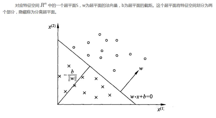
其中x為特征向量，w和b為感知機(jī)模型的參數(shù)。

感知機(jī)的幾何解釋：線性方程

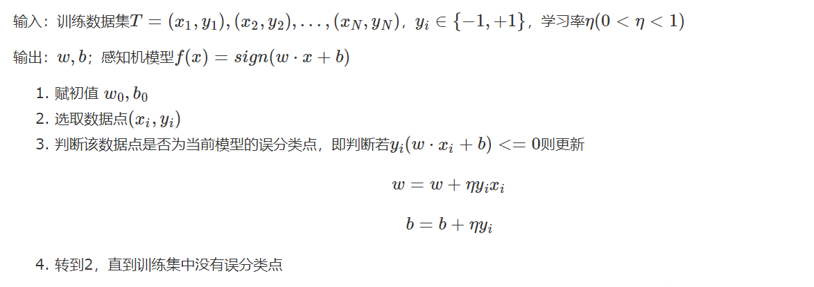
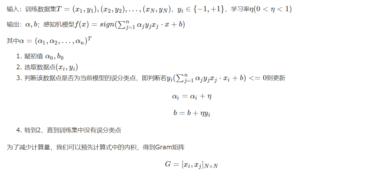
二·、感知機(jī)算法

1.原始形式

from random import randint
import numpy as np
import matplotlib.pyplot as plt


class TrainDataLoader:
    def __init__(self):
        pass
    def GenerateRandomData(self, count, gradient, offset):
        x1 = np.linspace(1, 5, count)
        x2 = gradient*x1 + np.random.randint(-10,10,*x1.shape)+offset
        dataset = []
        y = []
        for i in range(*x1.shape):
            dataset.append([x1[i], x2[i]])
            real_value = gradient*x1[i]+offset
            if real_value > x2[i]:
                y.append(-1)
            else:
                y.append(1)
        return x1,x2,np.mat(y),np.mat(dataset)


class SimplePerceptron:
    def __init__(self, train_data = [], real_result = [], eta = 1):
        self.w   =   np.zeros([1, len(train_data.T)], int)
        self.b   =   0
        self.eta =   eta
        self.train_data   = train_data
        self.real_result  = real_result
    def nomalize(self, x):
        if x > 0 :
            return 1
        else :
            return -1
    def model(self, x):
        # Here are matrix dot multiply get one value
        y = np.dot(x, self.w.T) + self.b
        # Use sign to nomalize the result
        predict_v = self.nomalize(y)
        return predict_v, y
    def update(self, x, y):
        # w = w + n*y_i*x_i
        self.w = self.w + self.eta*y*x
        # b = b + n*y_i
        self.b = self.b + self.eta*y
    def loss(slef, fx, y):
        return fx.astype(int)*y

    def train(self, count):
        update_count = 0
        while count > 0:
            # count--
            count = count - 1

            if len(self.train_data) <= 0:
                print("exception exit")
                break
            # random select one train data
            index = randint(0,len(self.train_data)-1)
            x = self.train_data[index]
            y = self.real_result.T[index]
            # wx+b
            predict_v, linear_y_v = self.model(x)
            # y_i*(wx+b) > 0, the classify is correct, else it's error
            if self.loss(y, linear_y_v) > 0:
                continue
            update_count = update_count + 1
            self.update(x, y)
        print("update count: ", update_count)
        pass
    def verify(self, verify_data, verify_result):
        size = len(verify_data)
        failed_count = 0
        if size <= 0:
            pass
        for i in range(size):
            x = verify_data[i]
            y = verify_result.T[i]
            if self.loss(y, self.model(x)[1]) > 0:
                continue
            failed_count = failed_count + 1
        success_rate = (1.0 - (float(failed_count)/size))*100
        print("Success Rate: ", success_rate, "%")
        print("All input: ", size, " failed_count: ", failed_count)

    def predict(self, predict_data):
        size = len(predict_data)
        result = []
        if size <= 0:
            pass
        for i in range(size):
            x = verify_data[i]
            y = verify_result.T[i]
            result.append(self.model(x)[0])
        return result



if __name__ == "__main__":
    # Init some parameters
    gradient = 2
    offset   = 10
    point_num = 1000
    train_num = 50000
    loader = TrainDataLoader()
    x, y, result, train_data =  loader.GenerateRandomData(point_num, gradient, offset)
    x_t, y_t, test_real_result, test_data =  loader.GenerateRandomData(100, gradient, offset)

    # First training
    perceptron = SimplePerceptron(train_data, result)
    perceptron.train(train_num)
    perceptron.verify(test_data, test_real_result)
    print("T1: w:", perceptron.w," b:", perceptron.b)

    # Draw the figure
    # 1. draw the (x,y) points
    plt.plot(x, y, "*", color='gray')
    plt.plot(x_t, y_t, "+")
    # 2. draw y=gradient*x+offset line
    plt.plot(x,x.dot(gradient)+offset, color="red")
    # 3. draw the line w_1*x_1 + w_2*x_2 + b = 0
    plt.plot(x, -(x.dot(float(perceptron.w.T[0]))+float(perceptron.b))/float(perceptron.w.T[1])
             , color='green')
    plt.show()

from random import randint
import numpy as np
import matplotlib.pyplot as plt


class TrainDataLoader:
    def __init__(self):
        pass
    def GenerateRandomData(self, count, gradient, offset):
        x1 = np.linspace(1, 5, count)
        x2 = gradient*x1 + np.random.randint(-10,10,*x1.shape)+offset
        dataset = []
        y = []
        for i in range(*x1.shape):
            dataset.append([x1[i], x2[i]])
            real_value = gradient*x1[i]+offset
            if real_value > x2[i]:
                y.append(-1)
            else:
                y.append(1)
        return x1,x2,np.mat(y),np.mat(dataset)


class SimplePerceptron:
    def __init__(self, train_data = [], real_result = [], eta = 1):
        self.alpha   =   np.zeros([train_data.shape[0], 1], int)
        self.w   =   np.zeros([1, train_data.shape[1]], int)
        self.b   =   0
        self.eta =   eta
        self.train_data   = train_data
        self.real_result  = real_result
        self.gram         = np.matmul(train_data[0:train_data.shape[0]], train_data[0:train_data.shape[0]].T)
    def nomalize(self, x):
        if x > 0 :
            return 1
        else :
            return -1
    def train_model(self, index):
        temp = 0
        y = self.real_result.T
        # Here are matrix dot multiply get one value
        for i in range(len(self.alpha)):
            alpha      = self.alpha[i]
            if alpha == 0:
                continue
            gram_value = self.gram[index].T[i]
            temp = temp + alpha*y[i]*gram_value
        y = temp + self.b
        # Use sign to nomalize the result
        predict_v = self.nomalize(y)
        return predict_v, y
    def verify_model(self, x):
        # Here are matrix dot multiply get one value
        y = np.dot(x, self.w.T) + self.b
        # Use sign to nomalize the result
        predict_v = self.nomalize(y)
        return predict_v, y
    def update(self, index, x, y):
        # alpha = alpha + 1
        self.alpha[index] = self.alpha[index] + 1
        # b = b + n*y_i
        self.b = self.b + self.eta*y
    def loss(slef, fx, y):
        return fx.astype(int)*y

    def train(self, count):
        update_count = 0
        train_data_num = self.train_data.shape[0]
        print("train_data:", self.train_data)
        print("Gram:",self.gram)
        while count > 0:
            # count--
            count = count - 1

            if train_data_num <= 0:
                print("exception exit")
                break
            # random select one train data
            index = randint(0, train_data_num-1)
            if index >= train_data_num:
                print("exceptrion get the index")
                break;
            x = self.train_data[index]
            y = self.real_result.T[index]
            # w = \sum_{i=1}^{N}\alpha_iy_iGram[i]
            # wx+b
            predict_v, linear_y_v = self.train_model(index)
            # y_i*(wx+b) > 0, the classify is correct, else it's error
            if self.loss(y, linear_y_v) > 0:
                continue
            update_count = update_count + 1
            self.update(index, x, y)

        for i in range(len(self.alpha)):
            x = self.train_data[i]
            y = self.real_result.T[i]
            self.w = self.w + float(self.alpha[i])*x*float(y)
        print("update count: ", update_count)
        pass
    def verify(self, verify_data, verify_result):
        size = len(verify_data)
        failed_count = 0
        if size <= 0:
            pass
        for i in range(size-1):
            x = verify_data[i]
            y = verify_result.T[i]
            if self.loss(y, self.verify_model(x)[1]) > 0:
                continue
            failed_count = failed_count + 1
        success_rate = (1.0 - (float(failed_count)/size))*100
        print("Success Rate: ", success_rate, "%")
        print("All input: ", size, " failed_count: ", failed_count)

    def predict(self, predict_data):
        size = len(predict_data)
        result = []
        if size <= 0:
            pass
        for i in range(size):
            x = verify_data[i]
            y = verify_result.T[i]
            result.append(self.model(x)[0])
        return result



if __name__ == "__main__":
    # Init some parameters
    gradient = 2
    offset   = 10
    point_num = 1000
    train_num = 1000
    loader = TrainDataLoader()
    x, y, result, train_data =  loader.GenerateRandomData(point_num, gradient, offset)
    x_t, y_t, test_real_result, test_data =  loader.GenerateRandomData(100, gradient, offset)
    # train_data = np.mat([[3,3],[4,3],[1,1]])
    # First training
    perceptron = SimplePerceptron(train_data, result)
    perceptron.train(train_num)
    perceptron.verify(test_data, test_real_result)
    print("T1: w:", perceptron.w," b:", perceptron.b)

    # Draw the figure
    # 1. draw the (x,y) points
    plt.plot(x, y, "*", color='gray')
    plt.plot(x_t, y_t, "+")
    # 2. draw y=gradient*x+offset line
    plt.plot(x,x.dot(gradient)+offset, color="red")
    # 3. draw the line w_1*x_1 + w_2*x_2 + b = 0
    plt.plot(x, -(x.dot(float(perceptron.w.T[0]))+float(perceptron.b))/float(perceptron.w.T[1])
             , color='green')
    plt.show()