R做線性回歸及檢驗(yàn)

使用R對(duì)內(nèi)置鳶尾花數(shù)據(jù)集iris（在R提示符下輸入iris回車可看到內(nèi)容）進(jìn)行回歸分析，自行選擇因變量和自變量，注意Species這個(gè)分類變量的處理方法

## 將iris數(shù)據(jù)加載進(jìn)來(lái)
attach(iris)
## 查看iris數(shù)據(jù)的整體情況
str(iris)
## 'data.frame':    150 obs. of  5 variables:
##  $ Sepal.Length: num  5.1 4.9 4.7 4.6 5 5.4 4.6 5 4.4 4.9 ...
##  $ Sepal.Width : num  3.5 3 3.2 3.1 3.6 3.9 3.4 3.4 2.9 3.1 ...
##  $ Petal.Length: num  1.4 1.4 1.3 1.5 1.4 1.7 1.4 1.5 1.4 1.5 ...
##  $ Petal.Width : num  0.2 0.2 0.2 0.2 0.2 0.4 0.3 0.2 0.2 0.1 ...
##  $ Species     : Factor w/ 3 levels "setosa","versicolor",..: 1 1 1 1 1 1 1 1 1 1 ...
可以看出，共有150個(gè)樣本，5個(gè)變量，前四個(gè)是數(shù)值型，第五個(gè)變量是因子型。
## 查看數(shù)據(jù)散點(diǎn)分布情況
pairs(iris[, 1:4], col = "blue")

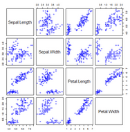
從上圖可以看出，Sepal.Length與Petal.Length、Petal.Length與Petal.Width存在明顯的正相關(guān)性。接下來(lái)選擇這兩對(duì)變量分別建立回歸模型。

(lm1 <- lm(Sepal.Length ~ Petal.Length))
## 
## Call:
## lm(formula = Sepal.Length ~ Petal.Length)
## 
## Coefficients:
##  (Intercept)  Petal.Length  
##        4.307         0.409
(lm2 <- lm(Petal.Length ~ Petal.Width))
## 
## Call:
## lm(formula = Petal.Length ~ Petal.Width)
## 
## Coefficients:
## (Intercept)  Petal.Width  
##        1.08         2.23
summary(lm1)
## 
## Call:
## lm(formula = Sepal.Length ~ Petal.Length)
## 
## Residuals:
##     Min      1Q  Median      3Q     Max 
## -1.2468 -0.2966 -0.0152  0.2768  1.0027 
## 
## Coefficients:
##              Estimate Std. Error t value Pr(>|t|)    
## (Intercept)    4.3066     0.0784    54.9   <2e-16 ***
## Petal.Length   0.4089     0.0189    21.6   <2e-16 ***
## ---
## Signif. codes:  0 '***' 0.001 '**' 0.01 '*' 0.05 '.' 0.1 ' ' 1
## 
## Residual standard error: 0.407 on 148 degrees of freedom
## Multiple R-squared:  0.76,   Adjusted R-squared:  0.758 
## F-statistic:  469 on 1 and 148 DF,  p-value: <2e-16
summary(lm2)
## 
## Call:
## lm(formula = Petal.Length ~ Petal.Width)
## 
## Residuals:
##     Min      1Q  Median      3Q     Max 
## -1.3354 -0.3035 -0.0295  0.2578  1.3945 
## 
## Coefficients:
##             Estimate Std. Error t value Pr(>|t|)    
## (Intercept)   1.0836     0.0730    14.8   <2e-16 ***
## Petal.Width   2.2299     0.0514    43.4   <2e-16 ***
## ---
## Signif. codes:  0 '***' 0.001 '**' 0.01 '*' 0.05 '.' 0.1 ' ' 1
## 
## Residual standard error: 0.478 on 148 degrees of freedom
## Multiple R-squared:  0.927,  Adjusted R-squared:  0.927 
## F-statistic: 1.88e+03 on 1 and 148 DF,  p-value: <2e-16
兩個(gè)模型的擬合效果都不錯(cuò)，但從R平方和角度考慮，lm2的模型效果好點(diǎn)。
##對(duì)建立的模型分別進(jìn)行殘差檢驗(yàn)
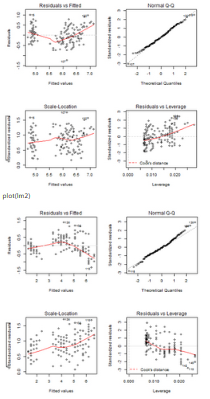
par(mfrow = c(2, 2))
plot(lm1)

par(mfrow = c(1, 2))
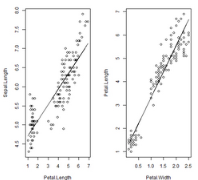
plot(Petal.Length, Sepal.Length)
lines(Petal.Length, lm1$fitted.values)
plot(Petal.Width, Petal.Length)
lines(Petal.Width, lm2$fitted.values)

數(shù)據(jù)中的第五個(gè)變量Species是因子型變量，在進(jìn)行回歸建模前，需要對(duì)其進(jìn)行啞變量處理，提高模型精確度。在R建立回歸模型時(shí)，會(huì)主動(dòng)對(duì)因子型變量進(jìn)行啞變量處理，下面先利用Sepal.Width、Species對(duì)Sepal.Length建立回歸模型，看看效果。

lm3 <- lm(Sepal.Length ~ Sepal.Width + Species)
summary(lm3)
## 
## Call:
## lm(formula = Sepal.Length ~ Sepal.Width + Species)
## 
## Residuals:
##     Min      1Q  Median      3Q     Max 
## -1.3071 -0.2571 -0.0533  0.1954  1.4125 
## 
## Coefficients:
##                   Estimate Std. Error t value Pr(>|t|)    
## (Intercept)          2.251      0.370    6.09  9.6e-09 ***
## Sepal.Width          0.804      0.106    7.56  4.2e-12 ***
## Speciesversicolor    1.459      0.112   13.01  < 2e-16 ***
## Speciesvirginica     1.947      0.100   19.47  < 2e-16 ***
## ---
## Signif. codes:  0 '***' 0.001 '**' 0.01 '*' 0.05 '.' 0.1 ' ' 1
## 
## Residual standard error: 0.438 on 146 degrees of freedom
## Multiple R-squared:  0.726,  Adjusted R-squared:  0.72 
## F-statistic:  129 on 3 and 146 DF,  p-value: <2e-16
par(mfrow = c(2, 2))
plot(lm3)

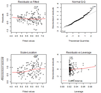
從建立的模型的各系數(shù)的p值看出，各參量均是顯著的。R平方和也有0.726，處于一個(gè)相對(duì)合理的水平。故該模型是可以接受的。

2 使用R對(duì)內(nèi)置longley數(shù)據(jù)集進(jìn)行回歸分析，如果以GNP.deflator作為因變量y，問(wèn)這個(gè)數(shù)據(jù)集是否存在多重共線性問(wèn)題？應(yīng)該選擇哪些變量參與回歸？

答：

## 查看longley的數(shù)據(jù)結(jié)構(gòu)
str(longley)
## 'data.frame':    16 obs. of  7 variables:
##  $ GNP.deflator: num  83 88.5 88.2 89.5 96.2 ...
##  $ GNP         : num  234 259 258 285 329 ...
##  $ Unemployed  : num  236 232 368 335 210 ...
##  $ Armed.Forces: num  159 146 162 165 310 ...
##  $ Population  : num  108 109 110 111 112 ...
##  $ Year        : int  1947 1948 1949 1950 1951 1952 1953 1954 1955 1956 ...
##  $ Employed    : num  60.3 61.1 60.2 61.2 63.2 ...
longly數(shù)據(jù)集中有7個(gè)變量16個(gè)觀測(cè)值，7個(gè)變量均屬于數(shù)值型。

首先建立全量回歸模型
lm1 <- lm(GNP.deflator ~ ., data = longley)
summary(lm1)
## 
## Call:
## lm(formula = GNP.deflator ~ ., data = longley)
## 
## Residuals:
##    Min     1Q Median     3Q    Max 
## -2.009 -0.515  0.113  0.423  1.550 
## 
## Coefficients:
##               Estimate Std. Error t value Pr(>|t|)  
## (Intercept)  2946.8564  5647.9766    0.52    0.614  
## GNP             0.2635     0.1082    2.44    0.038 *
## Unemployed      0.0365     0.0302    1.21    0.258  
## Armed.Forces    0.0112     0.0155    0.72    0.488  
## Population     -1.7370     0.6738   -2.58    0.030 *
## Year           -1.4188     2.9446   -0.48    0.641  
## Employed        0.2313     1.3039    0.18    0.863  
## ---
## Signif. codes:  0 '***' 0.001 '**' 0.01 '*' 0.05 '.' 0.1 ' ' 1
## 
## Residual standard error: 1.19 on 9 degrees of freedom
## Multiple R-squared:  0.993,  Adjusted R-squared:  0.988 
## F-statistic:  203 on 6 and 9 DF,  p-value: 4.43e-09
建立的模型結(jié)果是令人沮喪的，6個(gè)變量的顯著性p值只有兩個(gè)有一顆星，說(shuō)明有些變量不適合用于建模。

看各自變量是否存在共線性問(wèn)題。此處利用方差膨脹因子進(jìn)行判斷：方差膨脹因子VIF是指回歸系數(shù)的估計(jì)量由于自變量共線性使得方差增加的一個(gè)相對(duì)度量。一般建議，如VIF>10，表明模型中有很強(qiáng)的共線性問(wèn)題。
library(car)
vif(lm1, digits = 3)
##          GNP   Unemployed Armed.Forces   Population         Year 
##      1214.57        83.96        12.16       230.91      2065.73 
##     Employed 
##       220.42
從結(jié)果看，所有自變量的vif值均超過(guò)了10，其中GNP、Year更是高達(dá)四位數(shù)，存在嚴(yán)重的多種共線性。接下來(lái)，利用cor（）函數(shù)查看各自變量間的相關(guān)系數(shù)。
plot(longley[, 2:7])

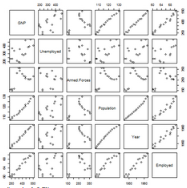
cor(longley[, 2:7])
##                 GNP Unemployed Armed.Forces Population   Year Employed
## GNP          1.0000     0.6043       0.4464     0.9911 0.9953   0.9836
## Unemployed   0.6043     1.0000      -0.1774     0.6866 0.6683   0.5025
## Armed.Forces 0.4464    -0.1774       1.0000     0.3644 0.4172   0.4573
## Population   0.9911     0.6866       0.3644     1.0000 0.9940   0.9604
## Year         0.9953     0.6683       0.4172     0.9940 1.0000   0.9713
## Employed     0.9836     0.5025       0.4573     0.9604 0.9713   1.0000
從散點(diǎn)分布圖和相關(guān)系數(shù)，均可以得知，自變量間存在嚴(yán)重共線性。
接下來(lái)利用step（）函數(shù)進(jìn)行變量的初步篩選。
lm1.step <- step(lm1, direction = "backward")
## Start:  AIC=10.48
## GNP.deflator ~ GNP + Unemployed + Armed.Forces + Population + 
##     Year + Employed
## 
##                Df Sum of Sq  RSS   AIC
## - Employed      1      0.04 12.9  8.54
## - Year          1      0.33 13.2  8.89
## - Armed.Forces  1      0.74 13.6  9.39
##                     12.8 10.48
## - Unemployed    1      2.08 14.9 10.88
## - GNP           1      8.47 21.3 16.59
## - Population    1      9.48 22.3 17.33
## 
## Step:  AIC=8.54
## GNP.deflator ~ GNP + Unemployed + Armed.Forces + Population + 
##     Year
## 
##                Df Sum of Sq  RSS   AIC
## - Year          1      0.46 13.3  7.11
##                     12.9  8.54
## - Armed.Forces  1      1.79 14.7  8.62
## - Unemployed    1      5.74 18.6 12.43
## - GNP           1      9.40 22.3 15.30
## - Population    1      9.90 22.8 15.66
## 
## Step:  AIC=7.11
## GNP.deflator ~ GNP + Unemployed + Armed.Forces + Population
## 
##                Df Sum of Sq  RSS   AIC
## - Armed.Forces  1       1.3 14.7  6.62
##                     13.4  7.11
## - Population    1       9.7 23.0 13.82
## - Unemployed    1      14.5 27.8 16.86
## - GNP           1      35.2 48.6 25.76
## 
## Step:  AIC=6.62
## GNP.deflator ~ GNP + Unemployed + Population
## 
##              Df Sum of Sq  RSS   AIC
##                   14.7  6.62
## - Unemployed  1      13.3 28.0 14.95
## - Population  1      13.3 28.0 14.95
## - GNP         1      48.6 63.2 27.99
根據(jù)AIC 赤池信息準(zhǔn)則，模型最后選擇Unemployed、Population、GNP三個(gè)因變量參與建模。
查看進(jìn)行逐步回歸后的模型效果
summary(lm1.step)
## 
## Call:
## lm(formula = GNP.deflator ~ GNP + Unemployed + Population, data = longley)
## 
## Residuals:
##    Min     1Q Median     3Q    Max 
## -2.047 -0.682  0.196  0.696  1.435 
## 
## Coefficients:
##              Estimate Std. Error t value Pr(>|t|)    
## (Intercept) 221.12959   48.97251    4.52  0.00071 ***
## GNP           0.22010    0.03493    6.30  3.9e-05 ***
## Unemployed    0.02246    0.00681    3.30  0.00634 ** 
## Population   -1.80501    0.54692   -3.30  0.00634 ** 
## ---
## Signif. codes:  0 '***' 0.001 '**' 0.01 '*' 0.05 '.' 0.1 ' ' 1
## 
## Residual standard error: 1.11 on 12 degrees of freedom
## Multiple R-squared:  0.992,  Adjusted R-squared:  0.989 
## F-statistic:  472 on 3 and 12 DF,  p-value: 1.03e-12
從各判定指標(biāo)可以看出，模型的結(jié)果是可喜的。參與建模的三個(gè)變量和截距均是顯著的。R平方和也高達(dá)0.992。