R語言繪圖學(xué)習(xí)筆記

在做數(shù)據(jù)分析時，我們通常作的舉動就是畫散點圖分析。因為通過散點圖的分析，我們可以最直觀，最簡單的得出大概的結(jié)論。今天我分享的內(nèi)容就是R語言的繪圖函數(shù)。

關(guān)于R語言強大的繪圖功能，我們可以通過函數(shù)demo(graphics),demo(persp)來見識R帶給我們的繪圖便利。

一、數(shù)據(jù)的初步分析
     我們對數(shù)據(jù)的初步分析常用的圖像有：散點圖、直方圖、莖葉圖、箱線圖。對于時間序列，散點圖，acf圖，pacf圖，殘差圖更是數(shù)據(jù)分析、建模的有利幫手。

先介紹創(chuàng)建圖像的函數(shù)plot（）的用法：

Plot（x,y…）:x（在x軸上）與y（在y軸上）的二元作圖，如果缺省x，x視為y的序列標(biāo)號

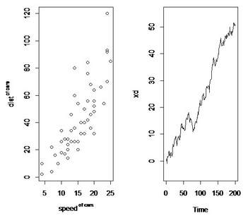
我們以截面數(shù)據(jù)（R中自帶數(shù)據(jù)集cars為例，看看散點圖的做法）

plot(cars$speed,cars$dist, xlab = expression(speed^" of cars"), ylab =expression(dist^" of cars"))#從圖中我們可以看到線性相關(guān)，從而可以考慮對這兩個變量做回歸分析

我們以隨機游走序列為例也來看一個時間序列圖：

set.seed(154)#用途是給定偽隨機數(shù)的seed，在同樣的seed下，R生成的偽隨機數(shù)序列是相同的。

w<-rnorm(200)

x<-cumsum(w)#累計求和，seeexample：cumsum(1:!0)

wd<-w+0.2

xd<-cumsum(wd)

plot.ts(xd,ylim=c(-5,55))

我們可以看到如下圖像：

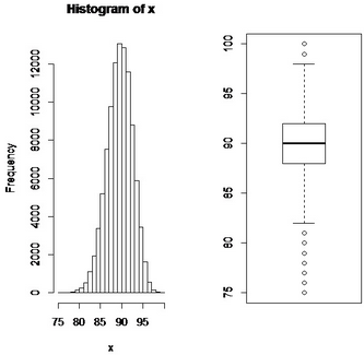
對于一些需要猜測分布截面數(shù)據(jù)，沒有比直方圖更適合的了。我們通常使用函數(shù)hist（）。用法如下：

hist(x, breaks = "Sturges",

freq = NULL, probability = !freq,

include.lowest = TRUE, right = TRUE,

density = NULL, angle = 45, col = NULL, border = NULL,

main = paste("Histogram of" , xname),

xlim = range(breaks), ylim = NULL,

xlab = xname, ylab,

axes = TRUE, plot = TRUE, labels = FALSE,

nclass = NULL, warn.unused = TRUE, ...)

我們來看看模擬二項分布所得的數(shù)據(jù)的畫出的直方圖：

x<-rbinom(100000,100,0.9)

hist(x)

通常對于大規(guī)模的數(shù)據(jù)，了解其分布也是需要的，我們常用箱線圖來描述，還是使用上面的模擬數(shù)據(jù)x,有boxplot(x).兩個函數(shù)得到的圖：

對于小規(guī)模數(shù)據(jù)，莖葉圖也是常被使用的。R中的stem函數(shù)可以完成它。Stem函數(shù)用法：stem(x, scale = 1, width = 80, atom = 1e-08)

>stem(log10(islands))#對于R的數(shù)據(jù)集islands取常用對數(shù)得到的莖葉圖.

The decimal point is at the |

1 | 1111112222233444

1 | 5555556666667899999

2 | 3344

2 | 59

3 |

3 | 5678

4 | 012

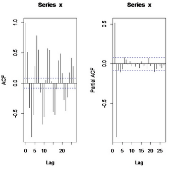
對于時間序列的繪圖，我們以AR（2）模型的模擬為例：

w<-rnorm(550)

x<-filter(w,filter=c(1,-0.9),"recursive")

acf(x)

pacf(x)

得到圖像：

這些可以創(chuàng)建一張圖的函數(shù)，在R中被稱為高級繪圖函數(shù)。除了我們提到的這些外還有餅圖：pie(),條形圖：barplot(),qq圖：qqnorm(),qqplot(),等高線：contour().等

二、圖像的內(nèi)容的豐富

R繪圖函數(shù)的大部分參數(shù)是一致的，主要參數(shù)有：

Add=F（默認(rèn)參數(shù)）：疊加圖形，不過要加點或線的話，一般使用points,lines這樣的低級繪圖函數(shù)

Type=”p” （默認(rèn)參數(shù)）：指定圖形類型：p：點,l：線,b：點連線,o：線在點上,h：垂直線,s：階梯式

Xlab,ylab:坐標(biāo)軸標(biāo)簽

Main：主標(biāo)題

Xlim,ylim:坐標(biāo)軸范圍

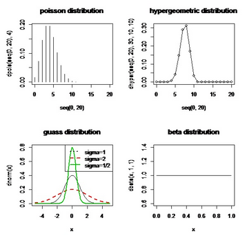
我們可以利用這些命令畫一些概率密度分布圖：

par(mfrow=c(2,2))

plot(seq(0,20),dpois(seq(0,20),4),type="h",main="poissondistribution")

plot(seq(0,20),dhyper(seq(0,20),30,10,10),type="o",main="hypergeometricdistribution")

curve(dnorm(x),xlim=c(-5,5),ylim=c(0,0.8))

curve(dnorm(x,0,2),add=T,col=2,lwd=2,lty=2)

curve(dnorm(x,0,1/2),add=T,col=3,lwd=2,lty=1)

legend(par('usr')[2],par('usr')[4],xjust=1,c("sigma=1","sigma=2","sigma=1/2"),

lwd=c(2,2,2),lty=c(3,2,1),col=c(1,2,3))

title(main="guassdistribution")

curve(dbeta(x,1,1),xlim=c(0,1),main="betadistribution")

得到圖像：

我們對上面用到的一些低級繪圖函數(shù)與繪圖參數(shù)做一個簡要說明：

Par（）：將圖像分為幾個部分，而且還可以指定每部分的長寬。如下例：

op<-par()

layout(matrix(c(2,1,0,3),2,2,byrow=T),c(1,6),c(4,1))

par(mar=c(1,1,5,2))

plot(cars$dist~cars$speed)

rug(side=1,jitter(cars$speed, 5))

rug(side=2,jitter(cars$dist, 5))

par(mar=c(1,2,5,1))

boxplot(cars$dist,axes=F)

par(op)#這個是在散點圖左側(cè)添加箱線圖，你可以直接運行它。

Col:設(shè)定顏色，可以用顏色的數(shù)字代號，也可以用顏色的英文

Legend:添加圖例，函數(shù)用法：

legend(x, y = NULL, legend, fill = NULL, col = par("col"),       border="black", lty, lwd, pch,       angle = 45, density = NULL, bty = "o", bg = par("bg"),       box.lwd = par("lwd"), box.lty = par("lty"), box.col = par("fg"),       pt.bg = NA, cex = 1, pt.cex = cex, pt.lwd = lwd,       xjust = 0, yjust = 1, x.intersp = 1, y.intersp = 1,       adj = c(0, 0.5), text.width = NULL, text.col = par("col"), text.font = NULL,       merge = do.lines && has.pch, trace = FALSE,       plot = TRUE, ncol = 1, horiz = FALSE, title = NULL,       inset = 0, xpd, title.col = text.col, title.adj = 0.5,       seg.len = 2)

Title:添加標(biāo)題，包括主標(biāo)題（main，置頂），副標(biāo)題（sub，置底）

Lty:控制連線類型

Lwd:控制連線寬度

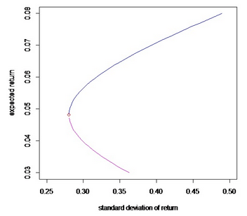
利用這些繪圖命令，我們也可以嘗試畫出資本市場線：

#portfolio_efficient_frontier

bmu<-array(c(0.08,0.03,0.05),dim=c(1,3))

bomega<-matrix(c(0.3,0.02,0.01,0.02,0.15,0.03,0.01,0.03,0.18),3,3)

bone<-t(as.matrix(rep(1,length(bmu))))

ibomega<-solve(bomega)

A<-as.numeric((bone)%*%ibomega%*%t(bmu))

B<-as.numeric((bmu)%*%ibomega%*%t(bmu))

C<-as.numeric((bone)%*%ibomega%*%t(bone))

D<-B*C-A*A

bg<-(B*ibomega%*%t(bone)-A*ibomega%*%t(bmu))/D

bh<-(C*ibomega%*%t(bmu)-A*ibomega%*%t(bone))/D

gg<-as.numeric(t(bg)%*%bomega%*%bg)

hh<-as.numeric(t(bh)%*%bomega%*%bh)

gh<-as.numeric(t(bg)%*%bomega%*%bh)

mumin<--as.numeric(gh)/as.numeric(hh)

sdmin<-as.numeric(sqrt(gg*(1-gh^2/gg/hh)))

muP<-seq(min(bmu),max(bmu),length=50)

sigmaP<-rep(0,50)

for(i in 1:50){

omegaP<-bg+muP[i]*bh

sigmaP[i]<-sqrt(t(omegaP)%*%bomega%*%omegaP)

}

ind<-(muP>mumin)

ind2<-(muP<mumin)

Ap<-sigmaP[ind]

Bp<-muP[ind]

Ap1<-sigmaP[ind2]

Bp1<-muP[ind2]

plot(Ap,Bp,ylim=c(0.03,0.08),xlim=c(0.25,0.5),type="l",col="blue",

xlab="standard deviation ofreturn",ylab="expected return")

points(sdmin,mumin,col="red")

lines(Ap1,Bp1,col=6)

如下圖：

還有一些繪圖函數(shù)，如text（），參數(shù)expression，在繪圖中也是十分重要的，但在此略去。

三、圖像的保存

這里我們默認(rèn)路徑為工作路徑，你可以通過getwd(),setwd()去查看或設(shè)置它。

其實在R語言里在圖形生成的窗口是可以通過單擊鼠標(biāo)右鍵來復(fù)制或保存圖像的，不過格式有限，通常是位圖。對于想要保存為其他格式的，可以通過如下命令：

第一種png格式

png(file="myplot.png",bg="transparent")

dev.off()

第二種jpeg格式

jpeg(file="myplot.jpeg")

dev.off()

文件都放在getwd()里了

第三種pdf格式

pdf(file="myplot.pdf")

dev.off()

下面是一個具體的例子

png(file="myplot.png",bg="transparent")

plot(1:10)

rect(1,5, 3, 7, col="white")

dev.off()

當(dāng)數(shù)據(jù)圖很多時，記得用paste（），

for(i ingenid){

pdf(file=paste(i,'.pdf',sep=''))

hist(get(i))

dev.off()

}

下面是我用jpeg格式保存的資本市場線，你可以與前面給出的位圖文件做一下對比：

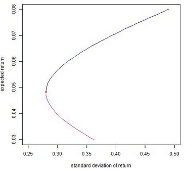
#這一次的R腳本文件  
    par(mfrow=c(1,2))  
      
    plot(cars$speed, cars$dist, xlab = expression(speed^" of cars"), ylab = expression(dist^" of cars"))  
      
    set.seed(154)#用途是給定偽隨機數(shù)的seed，在同樣的seed下，R生成的偽隨機數(shù)序列是相同的。這樣的話，別人的模擬就是可以重復(fù)的。  
    w<-rnorm(200)  
    x<-cumsum(w)#累計求和，see example：cumsum(1:!0)  
    wd<-w+0.2  
    xd<-cumsum(wd)  
    plot.ts(xd,ylim=c(-5,55))  
      
    x<-rbinom(100000,100,0.9)  
    hist(x)  
    boxplot(x)  
      
    stem(log10(islands))  
      
    w<-rnorm(550)  
    x<-filter(w,filter=c(1,-0.9),"recursive")  
    acf(x)  
    pacf(x)  
      
    par(mfrow=c(2,2))  
    plot(seq(0,20),dpois(seq(0,20),4),type="h",main="poisson distribution")  
    plot(seq(0,20),dhyper(seq(0,20),30,10,10),type="o",main="hypergeometric distribution")  
    curve(dnorm(x),xlim=c(-5,5),ylim=c(0,0.8))  
    curve(dnorm(x,0,2),add=T,col=2,lwd=2,lty=2)  
    curve(dnorm(x,0,1/2),add=T,col=3,lwd=2,lty=1)  
    legend(par('usr')[2],par('usr')[4],xjust=1,c("sigma=1","sigma=2","sigma=1/2"),  
    lwd=c(2,2,2),lty=c(3,2,1),col=c(1,2,3))  
    title(main="guass distribution")  
    curve(dbeta(x,1,1),xlim=c(0,1),main="beta distribution")  
      
    op<-par()  
    layout(matrix(c(2,1,0,3),2,2,byrow=T),c(1,6),c(4,1))  
    par(mar=c(1,1,5,2))  
    plot(cars$dist~cars$speed)  
    rug(side=1,jitter(cars$speed, 5))  
    rug(side=2,jitter(cars$dist, 5))  
    par(mar=c(1,2,5,1))  
    boxplot(cars$dist,axes=F)  
    par(op)  
      
    #portfolio_efficient_frontier  
    bmu<-array(c(0.08,0.03,0.05),dim=c(1,3))  
    bomega<-matrix(c(0.3,0.02,0.01,0.02,0.15,0.03,0.01,0.03,0.18),3,3)  
    bone<-t(as.matrix(rep(1,length(bmu))))  
    ibomega<-solve(bomega)  
    A<-as.numeric((bone)%*%ibomega%*%t(bmu))  
    B<-as.numeric((bmu)%*%ibomega%*%t(bmu))  
    C<-as.numeric((bone)%*%ibomega%*%t(bone))  
    D<-B*C-A*A  
    bg<-(B*ibomega%*%t(bone)-A*ibomega%*%t(bmu))/D  
    bh<-(C*ibomega%*%t(bmu)-A*ibomega%*%t(bone))/D  
      
    gg<-as.numeric(t(bg)%*%bomega%*%bg)  
    hh<-as.numeric(t(bh)%*%bomega%*%bh)  
    gh<-as.numeric(t(bg)%*%bomega%*%bh)  
    mumin<--as.numeric(gh)/as.numeric(hh)  
    sdmin<-as.numeric(sqrt(gg*(1-gh^2/gg/hh)))  
    muP<-seq(min(bmu),max(bmu),length=50)  
    sigmaP<-rep(0,50)  
    for(i in 1:50){  
    omegaP<-bg+muP[i]*bh  
    sigmaP[i]<-sqrt(t(omegaP)%*%bomega%*%omegaP)  
    }  
      
    ind<-(muP>mumin)  
    ind2<-(muP<mumin)  
      
    Ap<-sigmaP[ind]  
    Bp<-muP[ind]  
    Ap1<-sigmaP[ind2]  
    Bp1<-muP[ind2]  
    plot(Ap,Bp,ylim=c(0.03,0.08),xlim=c(0.25,0.5),type="l",col="blue",  
    xlab="standard deviation of return",ylab="expected return")  
    points(sdmin,mumin,col="red")  
    lines(Ap1,Bp1,col=6)