R語(yǔ)言與函數(shù)估計(jì)學(xué)習(xí)筆記（核方法與局部多項(xiàng)式）

非參數(shù)方法

用于函數(shù)估計(jì)的非參數(shù)方法大致上有三種：核方法、局部多項(xiàng)式方法、樣條方法。
非參的函數(shù)估計(jì)的優(yōu)點(diǎn)在于穩(wěn)健，對(duì)模型沒(méi)有什么特定的假設(shè)，只是認(rèn)為函數(shù)光滑，避免了模型選擇帶來(lái)的風(fēng)險(xiǎn)；但是，表達(dá)式復(fù)雜，難以解釋，計(jì)算量大是非參的一個(gè)很大的毛病。所以說(shuō)使用非參有風(fēng)險(xiǎn)，選擇需謹(jǐn)慎。
非參的想法很簡(jiǎn)單：函數(shù)在觀測(cè)到的點(diǎn)取觀測(cè)值的概率較大，用x附近的值通過(guò)加權(quán)平均的辦法估計(jì)函數(shù)f(x)的值。

核方法

當(dāng)加權(quán)的權(quán)重是某一函數(shù)的核（關(guān)于“核”的說(shuō)法可參見(jiàn)之前的博文《R語(yǔ)言與非參數(shù)統(tǒng)計(jì)（核密度估計(jì)）》）,這種方法就是核方法，常見(jiàn)的有Nadaraya-Watson核估計(jì)與Gasser-Muller核估計(jì)方法，也就是很多教材里談到的NW核估計(jì)與GM核估計(jì)，這里我們還是不談核的選擇，將一切的核估計(jì)都默認(rèn)用Gauss核處理。
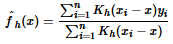
NW核估計(jì)形式為：

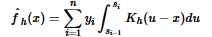
GM核估計(jì)形式為：

式中

x <- seq(-1, 1, length = 20)
y <- 5 * x * cos(5 * pi * x)
h <- 0.088
fx.hat <- function(z, h) {
    dnorm((z - x)/h)/h
}
KSMOOTH <- function(h, y, x) {
    n <- length(y)
    s.hat <- rep(0, n)
    for (i in 1:n) {
        a <- fx.hat(x[i], h)
        s.hat[i] <- sum(y * a/sum(a))
    }
    return(s.hat)
}

ksmooth.val <- KSMOOTH(h, y, x)

plot(x, y, xlab = "Predictor", ylab = "Response")
f <- function(x) 5 * x * cos(5 * pi * x)
curve(f, -1, 1, ylim = c(-15.5, 15.5), lty = 2, add = T)
lines(x, ksmooth.val, type = "l")

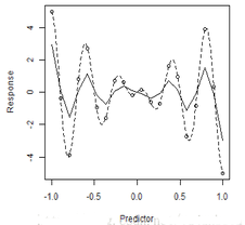
可以看出，核方法基本估計(jì)出了函數(shù)的形狀，但是效果不太好，這個(gè)是由于樣本點(diǎn)過(guò)少導(dǎo)致的，我們可以將樣本容量擴(kuò)大一倍，看看效果：

x <- seq(-1, 1, length = 40)
y <- 5 * x * cos(5 * pi * x)
h <- 0.055
fx.hat <- function(z, h) {
    dnorm((z - x)/h)/h
}
NWSMOOTH <- function(h, y, x) {
    n <- length(y)
    s.hat <- rep(0, n)
    for (i in 1:n) {
        a <- fx.hat(x[i], h)
        s.hat[i] <- sum(y * a/sum(a))
    }
    return(s.hat)
}

NWsmooth.val <- NWSMOOTH(h, y, x)

plot(x, y, xlab = "Predictor", ylab = "Response", col = 1)
f <- function(x) 5 * x * cos(5 * pi * x)
curve(f, -1, 1, ylim = c(-15.5, 15.5), lty = 1, add = T, col = 1)
lines(x, NWsmooth.val, lty = 2, col = 2)
A <- data.frame(x = seq(-1, 1, length = 1000))
model.linear <- lm(y ~ poly(x, 9))
lines(seq(-1, 1, length = 1000), predict(model.linear, A), lty = 3, col = 3)
letters <- c("NW method", "orignal model", "9 order poly-reg")
legend("bottomright", legend = letters, lty = c(2, 1, 3), col = c(2, 1, 3),
    cex = 0.5)

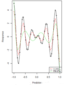
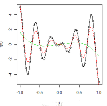
可以看到估計(jì)效果還是很好的，至少比基函數(shù)的辦法要好一些。那么我們來(lái)看看GM核方法：

x <- seq(-1, 1, length = 40)
y <- 5 * x * cos(5 * pi * x)
h <- 0.055

GMSMOOTH <- function(y, x, h) {
    n <- length(y)
    s <- c(-Inf, 0.5 * (x[-n] + x[-1]), Inf)
    s.hat <- rep(0, n)
    for (i in 1:n) {
        fx.hat <- function(z, h, x) {
            dnorm((x - z)/h)/h
        }
        a <- y[i] * integrate(fx.hat, s[i], s[i + 1], h = h, x = x[i])$value
        s.hat[i] <- sum(a)
    }
    return(s.hat)
}

GMsmooth.val <- GMSMOOTH(y, x, h)

plot(x, y, xlab = "Predictor", ylab = "Response", col = 1)
f <- function(x) 5 * x * cos(5 * pi * x)
curve(f, -1, 1, ylim = c(-15.5, 15.5), lty = 1, add = T, col = 1)
lines(x, GMsmooth.val, lty = 2, col = 2)
A <- data.frame(x = seq(-1, 1, length = 1000))
model.linear <- lm(y ~ poly(x, 9))
lines(seq(-1, 1, length = 1000), predict(model.linear, A), lty = 3, col = 3)
letters <- c("GM method", "orignal model", "9 order poly-reg")
legend("bottomright", legend = letters, lty = c(2, 1, 3), col = c(2, 1, 3),
    cex = 0.5)

我們來(lái)看看兩個(gè)核估計(jì)辦法的差異：

x <- seq(-1, 1, length = 40)
y <- 5 * x * cos(5 * pi * x)
h <- 0.055
fx.hat <- function(z, h) {
    dnorm((z - x)/h)/h
}
NWSMOOTH <- function(h, y, x) {
    n <- length(y)
    s.hat <- rep(0, n)
    for (i in 1:n) {
        a <- fx.hat(x[i], h)
        s.hat[i] <- sum(y * a/sum(a))
    }
    return(s.hat)
}

NWsmooth.val <- NWSMOOTH(h, y, x)

GMSMOOTH <- function(y, x, h) {
    n <- length(y)
    s <- c(-Inf, 0.5 * (x[-n] + x[-1]), Inf)
    s.hat <- rep(0, n)
    for (i in 1:n) {
        fx.hat <- function(z, h, x) {
            dnorm((x - z)/h)/h
        }
        a <- y[i] * integrate(fx.hat, s[i], s[i + 1], h = h, x = x[i])$value
        s.hat[i] <- sum(a)
    }
    return(s.hat)
}

GMsmooth.val <- GMSMOOTH(y, x, h)

plot(x, y, xlab = "Predictor", ylab = "Response", col = 1)
f <- function(x) 5 * x * cos(5 * pi * x)
curve(f, -1, 1, ylim = c(-15.5, 15.5), lty = 1, add = T, col = 1)
lines(x, NWsmooth.val, lty = 2, col = 2)
lines(x, GMsmooth.val, lty = 3, col = 3)
letters <- c("orignal model", "NW method", "GM method")
legend("bottomright", legend = letters, lty = 1:3, col = 1:3, cex = 0.5)

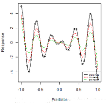
從圖中可以看到NW估計(jì)的方差似乎小些，事實(shí)也確實(shí)如此，GM估計(jì)的漸進(jìn)方差約為NW估計(jì)的1.5倍。但是GM估計(jì)解決了一些計(jì)算的難題。
我們最后還是來(lái)展示不同窗寬的選擇對(duì)估計(jì)的影響（這里以NW估計(jì)為例）：

x <- seq(-1, 1, length = 40)
y <- 5 * x * cos(5 * pi * x)
fx.hat <- function(z, h) {
    dnorm((z - x)/h)/h
}
NWSMOOTH <- function(h, y, x) {
    n <- length(y)
    s.hat <- rep(0, n)
    for (i in 1:n) {
        a <- fx.hat(x[i], h)
        s.hat[i] <- sum(y * a/sum(a))
    }
    return(s.hat)
}

h <- 0.025
NWsmooth.val0 <- NWSMOOTH(h, y, x)
h <- 0.05
NWsmooth.val1 <- NWSMOOTH(h, y, x)
h <- 0.1
NWsmooth.val2 <- NWSMOOTH(h, y, x)
h <- 0.2
NWsmooth.val3 <- NWSMOOTH(h, y, x)
h <- 0.3
NWsmooth.val4 <- NWSMOOTH(h, y, x)

plot(x, y, xlab = "Predictor", ylab = "Response", col = 1)
f <- function(x) 5 * x * cos(5 * pi * x)
curve(f, -1, 1, ylim = c(-15.5, 15.5), lty = 1, add = T, col = 1)
lines(x, NWsmooth.val0, lty = 2, col = 2)
lines(x, NWsmooth.val1, lty = 3, col = 3)
lines(x, NWsmooth.val2, lty = 4, col = 4)
lines(x, NWsmooth.val3, lty = 5, col = 5)
lines(x, NWsmooth.val4, lty = 6, col = 6)
letters <- c("orignal model", "h=0.025", "h=0.05", "h=0.1", "h=0.2", "h=0.3")
legend("bottom", legend = letters, lty = 1:6, col = 1:6, cex = 0.5)

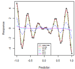
可以看到窗寬越大，估計(jì)越光滑，誤差越大，窗寬越小，估計(jì)越不光滑，但擬合優(yōu)度有提高，卻也容易過(guò)擬合。
窗寬怎么選，一個(gè)可行的辦法就是CV，通俗的講就是取一個(gè)觀測(cè)做測(cè)試集，剩下的做訓(xùn)練集，看NMSE。R代碼如下：

x <- seq(-1, 1, length = 40)
y <- 5 * x * cos(5 * pi * x)
# h<-0.055
NWSMOOTH <- function(h, y, x, z) {
    n <- length(y)
    s.hat <- rep(0, n)
    s.hat1 <- rep(0, n)
    for (i in 1:n) {
        s.hat[i] <- dnorm((x[i] - z)/h)/h * y[i]
        s.hat1[i] <- dnorm((x[i] - z)/h)/h
    }
    z.hat <- sum(s.hat)/sum(s.hat1)
    return(z.hat)
}
CVRSS <- function(h, y, x) {
    cv <- NULL
    for (i in seq(x)) {
        cv[i] <- (y[i] - NWSMOOTH(h, y[-i], x[-i], x[i]))^2
    }
    mean(cv)
}
h <- seq(0.01, 0.2, by = 0.005)
cvrss.val <- rep(0, length(h))
for (i in seq(h)) {
    cvrss.val[i] <- CVRSS(h[i], y, x)
}

plot(h, cvrss.val, type = "b")

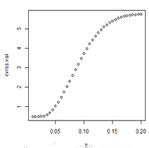
從圖中我們可以見(jiàn)到CV值在0.01到0.05的變化都不大，這時(shí)，我們應(yīng)該選擇較大的h，使得函數(shù)較為光滑，但是0.05后，cv變化較大，說(shuō)明我們選擇窗寬也不能過(guò)大，否則也會(huì)出毛病的。那么是不是h越小越好呢？雖然上面一個(gè)例子給了我們這樣一個(gè)錯(cuò)覺(jué)，我們下面這個(gè)例子就可以打破它，數(shù)據(jù)來(lái)自《computational statistics》一書(shū)的essay data一例。

easy <- read.table("D:/R/data/easysmooth.dat", header = T)
x <- easy$X
y <- easy$Y
NWSMOOTH <- function(h, y, x, z) {
    n <- length(y)
    s.hat <- rep(0, n)
    s.hat1 <- rep(0, n)
    for (i in 1:n) {
        s.hat[i] <- dnorm((x[i] - z)/h)/h * y[i]
        s.hat1[i] <- dnorm((x[i] - z)/h)/h
    }
    z.hat <- sum(s.hat)/sum(s.hat1)
    return(z.hat)
}
CVRSS <- function(h, y, x) {
    cv <- NULL
    for (i in seq(x)) {
        cv[i] <- (y[i] - NWSMOOTH(h, y[-i], x[-i], x[i]))^2
    }
    mean(cv)
}
h <- seq(0.01, 0.3, by = 0.02)
cvrss.val <- rep(0, length(h))
for (i in seq(h)) {
    cvrss.val[i] <- CVRSS(h[i], y, x)
}

plot(h, cvrss.val, type = "b")

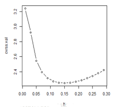
從上圖就可以看到，最佳窗寬約為0.15，而不是0.01.
和樹(shù)回歸類似，我們的核方法就是提供了一個(gè)常數(shù)來(lái)漸進(jìn)這個(gè)函數(shù)，我們這里仍然可以考慮模型樹(shù)的想法，用一階或者高階多項(xiàng)式來(lái)作加權(quán)估計(jì)，這就有了局部多項(xiàng)式估計(jì)。

局部多項(xiàng)式

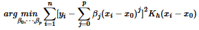
估計(jì)的想法是認(rèn)為未知函數(shù)f(x)在近鄰鄰域內(nèi)可由某一多項(xiàng)式近似（這是Taylor公式的結(jié)果），在x0的鄰域內(nèi)最小化：

具體做法為：
（1）對(duì)于每個(gè)xi，以該點(diǎn)為中心，計(jì)算出對(duì)應(yīng)點(diǎn)處的權(quán)重Kh(xi?x)；

（2）采用加權(quán)最小二乘法（WLS）估計(jì)其參數(shù)，并用得到的模型估計(jì)該結(jié)點(diǎn)對(duì)應(yīng)的x值對(duì)應(yīng)y值，作為y|xi的估計(jì)值（只要這一個(gè)點(diǎn)的估計(jì)值）；

（3）估計(jì)下一個(gè)點(diǎn)xj；

（4）將每個(gè)y|xi的估計(jì)值連接起來(lái)。
我們這里以《computational statistics》一書(shū)的essay data為例來(lái)說(shuō)明局部多項(xiàng)式估計(jì)

easy <- read.table("D:/R/data/easysmooth.dat", header = T)
x <- easy$X
y <- easy$Y
h <- 0.16

## FUNCTIONS USES HAT MATRIX

LPRSMOOTH <- function(y, x, h) {
    n <- length(y)
    s.hat <- rep(0, n)
    for (i in 1:n) {
        weight <- dnorm((x - x[i])/h)
        mod <- lm(y ~ x, weights = weight)
        s.hat[i] <- as.numeric(predict(mod, data.frame(x = x[i])))
    }
    return(s.hat)
}

lprsmooth.val <- LPRSMOOTH(y, x, h)

s <- function(x) {
    (x^3) * sin((x + 3.4)/2)
}
x.plot <- seq(min(x), max(x), length.out = 1000)
y.plot <- s(x.plot)
plot(x, y, xlab = "Predictor", ylab = "Response")
lines(x.plot, y.plot, lty = 1, col = 1)
lines(x, lprsmooth.val, lty = 2, col = 2)

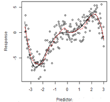
我們回到最開(kāi)始我們提到的三角函數(shù)的例子，我們可以看到：
x <- seq(-1, 1, length = 40)
y <- 5 * x * cos(5 * pi * x)

## FUNCTIONS


LPRSMOOTH <- function(y, x, h) {
    n <- length(y)
    s.hat <- rep(0, n)
    for (i in 1:n) {
        weight <- dnorm((x - x[i])/h)
        mod <- lm(y ~ x, weights = weight)
        s.hat[i] <- as.numeric(predict(mod, data.frame(x = x[i])))
    }
    return(s.hat)
}


h <- 0.15
lprsmooth.val1 <- LPRSMOOTH(y, x, h)


h <- 0.066
lprsmooth.val2 <- LPRSMOOTH(y, x, h)

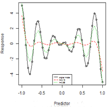
plot(x, y, xlab = "Predictor", ylab = "Response")
f <- function(x) 5 * x * cos(5 * pi * x)
curve(f, -1, 1, ylim = c(-15.5, 15.5), lty = 1, add = T, col = 1)
lines(x, lprsmooth.val1, lty = 2, col = 2)
lines(x, lprsmooth.val2, lty = 3, col = 3)
letters <- c("orignal model", "h=0.15", "h=0.66")
legend("bottom", legend = letters, lty = 1:3, col = 1:3, cex = 0.5

R中提供了很多的函數(shù)包來(lái)做非參數(shù)回歸，常用的有：KernSmooth包的函數(shù)locpoly()，locpol的locpol()，locCteSmootherC()以及l(fā)ocfit的locfit().具體的參數(shù)設(shè)置較為簡(jiǎn)單，這里就不多說(shuō)了。我們以開(kāi)篇的三角函數(shù)模型的例子為例來(lái)看看如何使用它們：

library(KernSmooth)  #函數(shù)locpoly()
library(locpol)  #locpol(); locCteSmootherC()
library(locfit)  #locfit()

x <- seq(-1, 1, length = 40)
y <- 5 * x * cos(5 * pi * x)

f <- function(x) 5 * x * cos(5 * pi * x)
curve(f, -1, 1)
points(x, y)

fit <- locpoly(x, y, bandwidth = 0.066)
lines(fit, lty = 2, col = 2)

d <- data.frame(x = x, y = y)
r <- locfit(y ~ x, d)  #一般來(lái)說(shuō)，locfit函數(shù)自動(dòng)選的窗寬偏大，函數(shù)較光滑
lines(r, lty = 3, col = 3)

xeval <- seq(-1, 1, length = 10)
cuest <- locCuadSmootherC(d$x, d$y, xeval, 0.066, gaussK)
cuest

##          x   beta0   beta1   beta2     den
## 1  -1.0000  5.0858 -35.152 -222.58 0.07571
## 2  -0.7778 -3.3233  11.966  514.42 4.22454
## 3  -0.5556  1.9804 -16.219 -279.47 4.26349
## 4  -0.3333 -0.8416  13.137   83.37 4.26349
## 5  -0.1111  0.1924  -4.983   27.90 4.26349
## 6   0.1111 -0.1924  -4.983  -27.90 4.26349
## 7   0.3333  0.8416  13.137  -83.37 4.26349
## 8   0.5556 -1.9804 -16.219  279.47 4.26349
## 9   0.7778  3.3233  11.966 -514.42 4.22454
## 10  1.0000 -5.0858 -35.152  222.58 0.07571

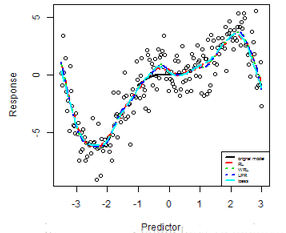
關(guān)于局部多項(xiàng)式估計(jì)的想法還有很多，比如我們只考慮近鄰的數(shù)據(jù)作最小二乘估計(jì)，再比如我們可以修改權(quán)重，使得我們的窗寬與近鄰點(diǎn)的距離有關(guān)，再比如，我們可以考慮不采用最小二乘做優(yōu)化，而是對(duì)最小二乘加上一點(diǎn)點(diǎn)的懲罰……我們將第一個(gè)想法稱之為running line，第二個(gè)想法稱之為loess,第三個(gè)想法依據(jù)你的懲罰方式不同有不同的說(shuō)法。我們將running line的R程序給出如下：

RLSMOOTH <- function(k, y, x) {
    n <- length(y)
    s.hat <- rep(0, n)
    b <- (k - 1)/2
    if (k > 1) {
        for (i in 1:(b + 1)) {
            xi <- x[1:(b + i)]
            xi <- cbind(rep(1, length(xi)), xi)
            hi <- xi %*% solve(t(xi) %*% xi) %*% t(xi)
            s.hat[i] <- y[1:(b + i)] %*% hi[i, ]

            xi <- x[(n - b - i + 1):n]
            xi <- cbind(rep(1, length(xi)), xi)
            hi <- xi %*% solve(t(xi) %*% xi) %*% t(xi)
            s.hat[n - i + 1] <- y[(n - b - i + 1):n] %*% hi[nrow(hi) - i + 1,
                ]
        }
        for (i in (b + 2):(n - b - 1)) {
            xi <- x[(i - b):(i + b)]
            xi <- cbind(rep(1, length(xi)), xi)
            hi <- xi %*% solve(t(xi) %*% xi) %*% t(xi)
            s.hat[i] <- y[(i - b):(i + b)] %*% hi[b + 1, ]
        }
    }
    if (k == 1) {
        s.hat <- y
    }
    return(s.hat)
}

我們也一樣可以對(duì)running line做局部多項(xiàng)式回歸，代碼如下：

WRLSMOOTH <- function(k, y, x, h) {
    n <- length(y)
    s.hat <- rep(0, n)
    b <- (k - 1)/2
    if (k > 1) {
        for (i in 1:(b + 1)) {
            xi <- x[1:(b + i)]
            xi <- cbind(rep(1, length(xi)), xi)
            hi <- xi %*% solve(t(xi) %*% xi) %*% t(xi)
            s.hat[i] <- y[1:(b + i)] %*% hi[i, ]

            xi <- x[(n - b - i + 1):n]
            xi <- cbind(rep(1, length(xi)), xi)
            hi <- xi %*% solve(t(xi) %*% xi) %*% t(xi)
            s.hat[n - i + 1] <- y[(n - b - i + 1):n] %*% hi[nrow(hi) - i + 1,
                ]
        }
        for (i in (b + 2):(n - b - 1)) {
            xi <- x[(i - b):(i + b)]
            weight <- dnorm((xi - x[i])/h)
            mod <- lm(y[(i - b):(i + b)] ~ xi, weights = weight)
            s.hat[i] <- as.numeric(predict(mod, data.frame(xi = x[i])))
        }
    }
    if (k == 1) {
        s.hat <- y
    }
    return(s.hat)
}

R中也提供了函數(shù)lowess()來(lái)做loess回歸。我們這里不妨以essay data為例，看看這三個(gè)估計(jì)有多大的差別：