使用Python一步一步地來進(jìn)行數(shù)據(jù)分析

你已經(jīng)決定來學(xué)習(xí)Python，但是你之前沒有編程經(jīng)驗(yàn)。因此，你常常對從哪兒著手而感到困惑，這么多Python的知識需要去學(xué)習(xí)。以下這些是那些開始使用Python數(shù)據(jù)分析的初學(xué)者的普遍遇到的問題：

    需要多久來學(xué)習(xí)Python？

    我需要學(xué)習(xí)Python到什么程度才能來進(jìn)行數(shù)據(jù)分析呢？

    學(xué)習(xí)Python最好的書或者課程有哪些呢？

    為了處理數(shù)據(jù)集，我應(yīng)該成為一個(gè)Python的編程專家嗎？

當(dāng)開始學(xué)習(xí)一項(xiàng)新技術(shù)時(shí)，這些都是可以理解的困惑。

不要害怕，我將會告訴你怎樣快速上手，而不必成為一個(gè)Python編程“忍者”。

不要犯我之前犯過的錯(cuò)

在開始使用Python之前，我對用Python進(jìn)行數(shù)據(jù)分析有一個(gè)誤解：我必須不得不對Python編程特別精通。我那會兒通過完成小的軟件項(xiàng)目來學(xué)習(xí)Python。敲代碼是快樂的事兒，但是我的目標(biāo)不是去成為一個(gè)Python開發(fā)人員，而是要使用Python數(shù)據(jù)分析。之后，我意識到，我花了很多時(shí)間來學(xué)習(xí)用Python進(jìn)行軟件開發(fā)，而不是數(shù)據(jù)分析。

在幾個(gè)小時(shí)的深思熟慮之后，我發(fā)現(xiàn)，我需要學(xué)習(xí)5個(gè)Python庫來有效地解決一系列的數(shù)據(jù)分析問題。然后，我開始一個(gè)接一個(gè)的學(xué)習(xí)這些庫。

在我看來,精通用Python開發(fā)好的軟件才能夠高效地進(jìn)行數(shù)據(jù)分析，這觀點(diǎn)是沒有必要的。

忽略給大眾的資源

有許多優(yōu)秀的Python書籍和在線課程，然而我不并不推薦它們中的一些，因?yàn)?，有些是給大眾準(zhǔn)備的而不是給那些用來數(shù)據(jù)分析的人準(zhǔn)備的。同樣也有許多書是“用Python科學(xué)編程”的，但它們是面向各種數(shù)學(xué)為導(dǎo)向的主題的，而不是成為為了數(shù)據(jù)分析和統(tǒng)計(jì)。不要浪費(fèi)浪費(fèi)你的時(shí)間去閱讀那些為大眾準(zhǔn)備的Python書籍。
在進(jìn)一步繼續(xù)之前，首先設(shè)置好你的編程環(huán)境，然后學(xué)習(xí)怎么使用IPython notebook

Numpy

首先，開始學(xué)習(xí)Numpy吧，因?yàn)樗抢肞ython科學(xué)計(jì)算的基礎(chǔ)包。對Numpy好的掌握將會幫助你有效地使用其他工具例如Pandas。

我已經(jīng)準(zhǔn)備好了IPython筆記，這包含了Numpy的一些基本概念。這個(gè)教程包含了Numpy中最頻繁使用的操作，例如，N維數(shù)組，索引，數(shù)組切片，整數(shù)索引，數(shù)組轉(zhuǎn)換，通用函數(shù)，使用數(shù)組處理數(shù)據(jù)，常用的統(tǒng)計(jì)方法，等等。

Pandas包含了高級的數(shù)據(jù)結(jié)構(gòu)和操作工具，它們使得Python數(shù)據(jù)分析更加快速和容易。
教程包含了series, data frams，從一個(gè)axis刪除數(shù)據(jù)，缺失數(shù)據(jù)處理，等等。
Matplotlib

這是一個(gè)分為四部分的Matplolib教程。
1st 部分:

第一部分介紹了Matplotlib基本功能，基本figure類型。

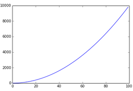
Simple Plotting example

In [113]:

%matplotlib inline
import matplotlib.pyplot as plt #importing matplot lib libraryimport
 numpy as np
x = range(100)
#print x, print and check what is xy =[val**2 for val in x]
#print yplt.plot(x,y) #plotting x and y

Out[113]:

[<matplotlib.lines.Line2D at 0x7857bb0>]

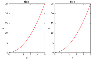
fig, axes = plt.subplots(nrows=1, ncols=2)for ax in axes:    ax.plot(x, y, 'r')    ax.set_xlabel('x')    ax.set_ylabel('y')    ax.set_title('title')    fig.tight_layout()

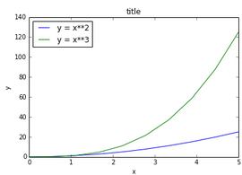
fig, ax = plt.subplots()ax.plot(x, x**2, label="y = x**2")ax.plot(x, x**3,
label="y = x**3")ax.legend(loc=2); # upper left cornerax.set_xlabel('x')
ax.set_ylabel('y')ax.set_title('title');

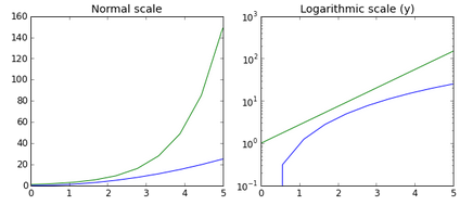
fig, axes = plt.subplots(1, 2, figsize=(10,4))    
  axes[0].plot(x, x**2, x, np.exp(x))axes[0].set_title("Normal scale")
axes[1].plot(x, x**2, x, np.exp(x))axes[1].set_yscale("log")axes[1].set_title
("Logarithmic scale (y)");

n = np.array([0,1,2,3,4,5])

In [47]:

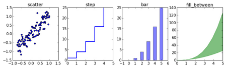
fig, axes = plt.subplots(1, 4, figsize=(12,3))axes[0].scatter
(xx, xx + 0.25*np.random.randn(len(xx)))axes[0].set_title("scatter")axes[1].step
(n, n**2, lw=2)axes[1].set_title("step")axes[2].bar(n, n**2, align="center",
width=0.5, alpha=0.5)axes[2].set_title("bar")axes[3].fill_between(x, x**2, x**3,
color="green", alpha=0.5);axes[3].set_title("fill_between");

Using Numpy

In [17]:

x = np.linspace(0, 2*np.pi, 100)y =np.sin(x)plt.plot(x,y)

Out[17]:

[<matplotlib.lines.Line2D at 0x579aef0>]
In [24]:

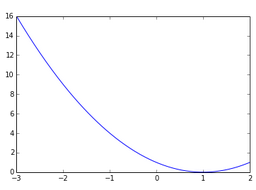
x= np.linspace(-3,2, 200)Y = x ** 2 - 2 * x + 1.plt.plot(x,Y)

Out[24]:

[<matplotlib.lines.Line2D at 0x6ffb310>]

In [32]:

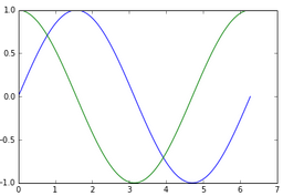
# plotting multiple plotsx =np.linspace(0, 2 * np.pi, 100)y = np.sin(x)z =
np.cos(x)plt.plot(x,y)
plt.plot(x,z)plt.show()# Matplot lib picks different colors for different plot.

In [35]:

cd C:\Users\tk\Desktop\Matplot
C:\Users\tk\Desktop\Matplot

In [39]:

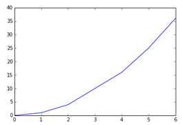
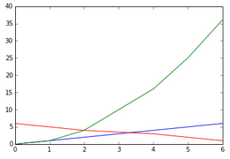
data = np.loadtxt('numpy.txt')plt.plot(data[:,0], data[:,1]) # plotting column
1 vs column 2# The text in the numpy.txt should look like this
# 0 0# 1 1# 2 4# 4 16# 5 25# 6 36

Out[39]:

[<matplotlib.lines.Line2D at 0x740f090>]

In [56]:

data1 = np.loadtxt('scipy.txt') # load the fileprint data1.Tfor val in data1.T:
#loop over each and every value in data1.T    plt.plot(data1[:,0], val)
#data1[:,0] is the first row in data1.T    # data in scipy.txt looks like this:
# 0 0  6# 1 1  5# 2 4  4
# 4 16 3# 5 25 2# 6 36 1

[[  0.   1.   2.   4.   5.   6.]
 [  0.   1.   4.  16.  25.  36.]
 [  6.   5.   4.   3.   2.   1.]]

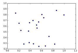
Scatter Plots and Bar Graphs

In [64]:

sct = np.random.rand(20, 2)print sctplt.scatter(sct[:,0], sct[:,1])
# I am plotting a scatter plot.

[[ 0.51454542  0.61859101]
 [ 0.45115993  0.69774873]
 [ 0.29051205  0.28594808]
 [ 0.73240446  0.41905186]
 [ 0.23869394  0.5238878 ]
 [ 0.38422814  0.31108919]
 [ 0.52218967  0.56526379]
 [ 0.60760426  0.80247073]
 [ 0.37239096  0.51279078]
 [ 0.45864677  0.28952167]
 [ 0.8325996   0.28479446]
 [ 0.14609382  0.8275477 ]
 [ 0.86338279  0.87428696]
 [ 0.55481585  0.24481165]
 [ 0.99553336  0.79511137]
 [ 0.55025277  0.67267026]
 [ 0.39052024  0.65924857]
 [ 0.66868207  0.25186664]
 [ 0.64066313  0.74589812]
 [ 0.20587731  0.64977807]]

Out[64]:

<matplotlib.collections.PathCollection at 0x78a7110>

In [65]:

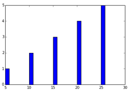
ghj =[5, 10 ,15, 20, 25]it =[ 1, 2, 3, 4, 5]plt.bar(ghj, it) # simple bar graph

Out[65]:

<Container object of 5 artists>

In [74]:

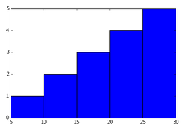
ghj =[5, 10 ,15, 20, 25]it =[ 1, 2, 3, 4, 5]plt.bar(ghj, it, width =5)# you can change the thickness of a bar, by default the bar will have a thickness of 0.8 units

Out[74]:

<Container object of 5 artists>

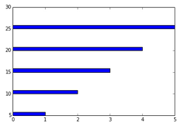
In [75]:

ghj =[5, 10 ,15, 20, 25]it =[ 1, 2, 3, 4, 5]plt.barh(ghj, it) # barh is a horizontal bar graph

Out[75]:

<Container object of 5 artists>

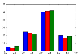
Multiple bar charts

In [95]:

new_list = [[5., 25., 50., 20.], [4., 23., 51., 17.], [6., 22., 52., 19.]]x = np.arange(4)
plt.bar(x + 0.00, new_list[0], color ='b', width =0.25)plt.bar(x + 0.25, new_list[1], color ='r', width =0.25)plt.bar(x + 0.50, new_list[2], color ='g', width =0.25)#plt.show()

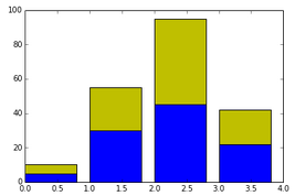
In [100]:

#Stacked Bar chartsp = [5., 30., 45., 22.]q = [5., 25., 50., 20.]
x =range(4)plt.bar(x, p, color ='b')plt.bar(x, q, color ='y', bottom =p)

Out[100]:

<Container object of 4 artists>

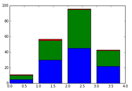
In [35]:

# plotting more than 2 valuesA = np.array([5., 30., 45., 22.])
B = np.array([5., 25., 50., 20.])C = np.array([1., 2., 1., 1.])
X = np.arange(4)plt.bar(X, A, color = 'b')plt.bar(X, B, color = 'g', bottom = A)plt.bar(X, C, color = 'r', bottom = A + B) # for the third argument, I use A+Bplt.show()

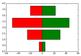
In [94]:

black_money = np.array([5., 30., 45., 22.])
white_money = np.array([5., 25., 50., 20.])z = np.arange(4)plt.barh(z, black_money, color ='g')plt.barh(z, -white_money, color ='r')# - notation is needed for generating, back to back charts

Out[94]:

<Container object of 4 artists>

Other Plots

In [114]:

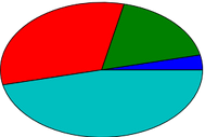
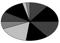
#Pie chartsy = [5, 25, 45, 65]plt.pie(y)

Out[114]:

([<matplotlib.patches.Wedge at 0x7a19d50>,
  <matplotlib.patches.Wedge at 0x7a252b0>,
  <matplotlib.patches.Wedge at 0x7a257b0>,
  <matplotlib.patches.Wedge at 0x7a25cb0>],
 [<matplotlib.text.Text at 0x7a25070>,
  <matplotlib.text.Text at 0x7a25550>,
  <matplotlib.text.Text at 0x7a25a50>,
  <matplotlib.text.Text at 0x7a25f50>])
 
In [115]:

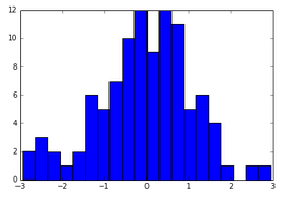
#Histogramsd = np.random.randn(100)plt.hist(d, bins = 20)

Out[115]:

(array([  2.,   3.,   2.,   1.,   2.,   6.,   5.,   7.,  10.,  12.,   9.,
         12.,  11.,   5.,   6.,   4.,   1.,   0.,   1.,   1.]),
 array([-2.9389701 , -2.64475645, -2.35054281, -2.05632916, -1.76211551,
        -1.46790186, -1.17368821, -0.87947456, -0.58526092, -0.29104727,
         0.00316638,  0.29738003,  0.59159368,  0.88580733,  1.18002097,
         1.47423462,  1.76844827,  2.06266192,  2.35687557,  2.65108921,
         2.94530286]),
 <a list of 20 Patch objects>)

In [116]:

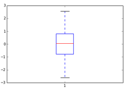
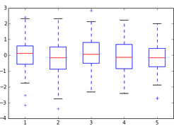
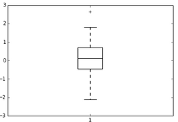
d = np.random.randn(100)plt.boxplot(d)#1) The red bar is the median of the distribution#2) The blue box includes 50 percent of the data from the lower quartile to the upper quartile.
#   Thus, the box is centered on the median of the data.

Out[116]:

{'boxes': [<matplotlib.lines.Line2D at 0x7cca090>],
 'caps': [<matplotlib.lines.Line2D at 0x7c02d70>,
  <matplotlib.lines.Line2D at 0x7cc2c90>],
 'fliers': [<matplotlib.lines.Line2D at 0x7cca850>,
  <matplotlib.lines.Line2D at 0x7ccae10>],
 'medians': [<matplotlib.lines.Line2D at 0x7cca470>],
 'whiskers': [<matplotlib.lines.Line2D at 0x7c02730>,
  <matplotlib.lines.Line2D at 0x7cc24b0>]}

In [118]:

d = np.random.randn(100, 5) # generating multiple box plotsplt.boxplot(d)

Out[118]:

{'boxes': [<matplotlib.lines.Line2D at 0x7f49d70>,
  <matplotlib.lines.Line2D at 0x7ea1c90>,
  <matplotlib.lines.Line2D at 0x7eafb90>,
  <matplotlib.lines.Line2D at 0x7ebea90>,
  <matplotlib.lines.Line2D at 0x7ece990>],
 'caps': [<matplotlib.lines.Line2D at 0x7f2b3b0>,
  <matplotlib.lines.Line2D at 0x7f49990>,
  <matplotlib.lines.Line2D at 0x7ea14d0>,
  <matplotlib.lines.Line2D at 0x7ea18b0>,
  <matplotlib.lines.Line2D at 0x7eaf3d0>,
  <matplotlib.lines.Line2D at 0x7eaf7b0>,
  <matplotlib.lines.Line2D at 0x7ebe2d0>,
  <matplotlib.lines.Line2D at 0x7ebe6b0>,
  <matplotlib.lines.Line2D at 0x7ece1d0>,
  <matplotlib.lines.Line2D at 0x7ece5b0>],
 'fliers': [<matplotlib.lines.Line2D at 0x7e98550>,
  <matplotlib.lines.Line2D at 0x7e98930>,
  <matplotlib.lines.Line2D at 0x7ea8470>,
  <matplotlib.lines.Line2D at 0x7ea8a10>,
  <matplotlib.lines.Line2D at 0x7eb6370>,
  <matplotlib.lines.Line2D at 0x7eb6730>,
  <matplotlib.lines.Line2D at 0x7ec6270>,
  <matplotlib.lines.Line2D at 0x7ec6810>,
  <matplotlib.lines.Line2D at 0x8030170>,
  <matplotlib.lines.Line2D at 0x8030710>],
 'medians': [<matplotlib.lines.Line2D at 0x7e98170>,
  <matplotlib.lines.Line2D at 0x7ea8090>,
  <matplotlib.lines.Line2D at 0x7eaff70>,
  <matplotlib.lines.Line2D at 0x7ebee70>,
  <matplotlib.lines.Line2D at 0x7eced70>],
 'whiskers': [<matplotlib.lines.Line2D at 0x7f2bb50>,
  <matplotlib.lines.Line2D at 0x7f491b0>,
  <matplotlib.lines.Line2D at 0x7e98cf0>,
  <matplotlib.lines.Line2D at 0x7ea10f0>,
  <matplotlib.lines.Line2D at 0x7ea8bf0>,
  <matplotlib.lines.Line2D at 0x7ea8fd0>,
  <matplotlib.lines.Line2D at 0x7eb6cd0>,
  <matplotlib.lines.Line2D at 0x7eb6ed0>,
  <matplotlib.lines.Line2D at 0x7ec6bd0>,
  <matplotlib.lines.Line2D at 0x7ec6dd0>]}

MatplotLib Part 1
2nd 部分:

包含了怎么調(diào)整figure的樣式和顏色，例如：makers,line,thicness,line patterns和color map.

%matplotlib inlineimport numpy as npimport matplotlib.pyplot as plt

In [22]:

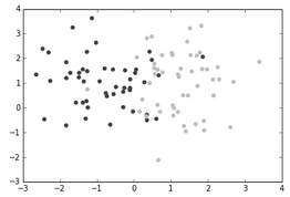
p =np.random.standard_normal((50,2))p += np.array((-1,1)) # center the distribution at (-1,1)q =np.random.standard_normal((50,2))q += np.array((1,1)) #center the distribution at (-1,1)plt.scatter(p[:,0], p[:,1], color ='.25')plt.scatter(q[:,0], q[:,1], color = '.75')

Out[22]:

<matplotlib.collections.PathCollection at 0x71dab90>

In [34]:

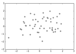
dd =np.random.standard_normal((50,2))plt.scatter(dd[:,0], dd[:,1], color ='1.0', edgecolor ='0.0') # edge color controls the color of the edge

Out[34]:

<matplotlib.collections.PathCollection at 0x7336670>

Custom Color for Bar charts,Pie charts and box plots:
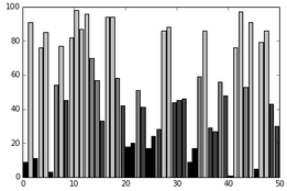
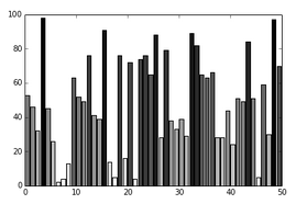
The below bar graph, plots x(1 to 50) (vs) y(50 random integers, within 0-100. But you need different colors for each value. For which we create a list containing four colors(color_set). The list comprehension creates 50 different color values from color_set

In [9]:

vals = np.random.random_integers(99, size =50)color_set = ['.00', '.25', '.50','.75']color_lists = [color_set[(len(color_set)* val) // 100] for val in vals]c = plt.bar(np.arange(50), vals, color = color_lists)

In [8]:

hi =np.random.random_integers(8, size =10)color_set =['.00', '.25', '.50', '.75']plt.pie(hi, colors = color_set)# colors attribute accepts a range of valuesplt.show()#If there are less colors than values, then pyplot.pie() will simply cycle through the color list. In the preceding
#example, we gave a list of four colors to color a pie chart that consisted of eight values. Thus, each color will be used twice

In [27]:
values = np.random.randn(100)w = plt.boxplot(values)for att, lines in w.iteritems():    for l in lines:        l.set_color('k')

Color Maps
 
know more about hsv

In [34]:

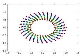
# how to color scatter plots#Colormaps are defined in the matplotib.cm module. This module provides
#functions to create and use colormaps. It also provides an exhaustive choice of predefined color maps.import matplotlib.cm as cmN = 256angle = np.linspace(0, 8 * 2 * np.pi, N)radius = np.linspace(.5, 1., N)X = radius * np.cos(angle)Y = radius * np.sin(angle)plt.scatter(X,Y, c=angle, cmap = cm.hsv)

Out[34]:

<matplotlib.collections.PathCollection at 0x714d9f0>

In [44]:

#Color in bar graphsimport matplotlib.cm as cmvals = np.random.random_integers(99, size =50)cmap = cm.ScalarMappable(col.Normalize(0,99), cm.binary)plt.bar(np.arange(len(vals)),vals, color =cmap.to_rgba(vals))

Out[44]:

<Container object of 50 artists>
 
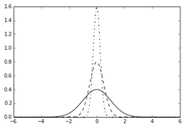
Line Styles

In [4]:

# I am creating 3 levels of gray plots, with different line shades

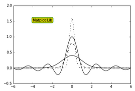
def pq(I, mu, sigma):    a = 1. / (sigma * np.sqrt(2. * np.pi))    b = -1. / (2. * sigma ** 2)    return a * np.exp(b * (I - mu) ** 2)I =np.linspace(-6,6, 1024)plt.plot(I, pq(I, 0., 1.), color = 'k', linestyle ='solid')plt.plot(I, pq(I, 0., .5), color = 'k', linestyle ='dashed')plt.plot(I, pq(I, 0., .25), color = 'k', linestyle ='dashdot')

Out[4]:

[<matplotlib.lines.Line2D at 0x562ffb0>]

 

In [12]:

N = 15A = np.random.random(N)B= np.random.random(N)X = np.arange(N)plt.bar(X, A, color ='.75')plt.bar(X, A+B , bottom = A, color ='W', linestyle ='dashed') # plot a bar graphplt.show()

 

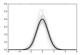
In [20]:

def gf(X, mu, sigma):    a = 1. / (sigma * np.sqrt(2. * np.pi))    b = -1. / (2. * sigma ** 2)    return a * np.exp(b * (X - mu) ** 2)X = np.linspace(-6, 6, 1024)for i in range(64):    samples = np.random.standard_normal(50)    mu,sigma = np.mean(samples), np.std(samples)    plt.plot(X, gf(X, mu, sigma), color = '.75', linewidth = .5)plt.plot(X, gf(X, 0., 1.), color ='.00', linewidth = 3.)

Out[20]:

[<matplotlib.lines.Line2D at 0x59fbab0>]

 

 
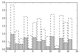
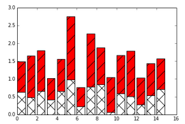
Fill surfaces with pattern

In [27]:

N = 15A = np.random.random(N)B= np.random.random(N)X = np.arange(N)plt.bar(X, A, color ='w', hatch ='x')plt.bar(X, A+B,bottom =A, color ='r', hatch ='/')# some other hatch attributes are :#/#\#|#-#+#x#o#O#.#*

Out[27]:

<Container object of 15 artists>

 

 
Marker styles

In [29]:

cd C:\Users\tk\Desktop\Matplot

 

C:\Users\tk\Desktop\Matplot

 
Come back to this section later

In [14]:

X= np.linspace(-6,6,1024)Ya =np.sinc(X)Yb = np.sinc(X) +1plt.plot(X, Ya, marker ='o', color ='.75')plt.plot(X, Yb, marker ='^', color='.00', markevery= 32)# this one marks every 32 nd element

Out[14]:

[<matplotlib.lines.Line2D at 0x7063150>]

 
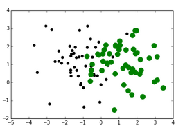
In [31]:

# Marker SizeA = np.random.standard_normal((50,2))A += np.array((-1,1))B = np.random.standard_normal((50,2))B += np.array((1, 1))plt.scatter(A[:,0], A[:,1], color ='k', s =25.0)plt.scatter(B[:,0], B[:,1], color ='g', s = 100.0) # size of the marker is specified using 's' attribute

Out[31]:

<matplotlib.collections.PathCollection at 0x7d015f0>

Own Marker Shapes- come back to this later

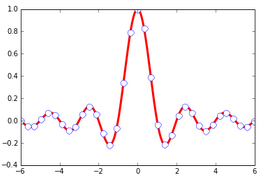
In [65]:

# more about markersX =np.linspace(-6,6, 1024)Y =np.sinc(X)plt.plot(X,Y, color ='r', marker ='o', markersize =9, markevery = 30, markerfacecolor='w', linewidth = 3.0, markeredgecolor = 'b')

Out[65]:

[<matplotlib.lines.Line2D at 0x84c9750>]

In [20]:

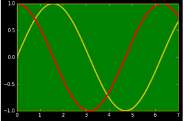
import matplotlib as mplmpl.rc('lines', linewidth =3)mpl.rc('xtick', color ='w') # color of x axis numbersmpl.rc('ytick', color = 'w') # color of y axis numbersmpl.rc('axes', facecolor ='g', edgecolor ='y') # color of axes
mpl.rc('figure', facecolor ='.00',edgecolor ='w') # color of figurempl.rc('axes', color_cycle = ('y','r')) # color of plotsx = np.linspace(0, 7, 1024)plt.plot(x, np.sin(x))plt.plot(x, np.cos(x))

Out[20]:

[<matplotlib.lines.Line2D at 0x7b0fb70>]

MatplotLib Part2
3rd 部分:

圖的注釋--包含若干圖，控制坐標(biāo)軸范圍，長款比和坐標(biāo)軸。
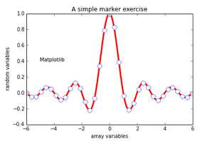
Annotation

In [1]:

%matplotlib inlineimport numpy as npimport matplotlib.pyplot as plt

In [28]:

X =np.linspace(-6,6, 1024)Y =np.sinc(X)plt.title('A simple marker exercise')# a title notationplt.xlabel('array variables') # adding xlabelplt.ylabel(' random variables') # adding ylabelplt.text(-5, 0.4, 'Matplotlib') # -5 is the x value and 0.4 is y valueplt.plot(X,Y, color ='r', marker ='o', markersize =9, markevery = 30, markerfacecolor='w', linewidth = 3.0, markeredgecolor = 'b')

Out[28]:

[<matplotlib.lines.Line2D at 0x84b6430>]

In [39]:

def pq(I, mu, sigma):    a = 1. / (sigma * np.sqrt(2. * np.pi))    b = -1. / (2. * sigma ** 2)    return a * np.exp(b * (I - mu) ** 2)I =np.linspace(-6,6, 1024)plt.plot(I, pq(I, 0., 1.), color = 'k', linestyle ='solid')plt.plot(I, pq(I, 0., .5), color = 'k', linestyle ='dashed')plt.plot(I, pq(I, 0., .25), color = 'k', linestyle ='dashdot')# I have created a dictinary of stylesdesign = {'facecolor' : 'y', # color used for the text box'edgecolor' : 'g',
'boxstyle' : 'round'
}plt.text(-4, 1.5, 'Matplot Lib', bbox = design)plt.plot(X, Y, c='k')plt.show()

#This sets the style of the box, which can either be 'round' or 'square'
#'pad': If 'boxstyle' is set to 'square', it defines the amount of padding between the text and the box's sides

Alignment Control

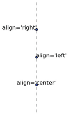
The text is bound by a box. This box is used to relatively align the text to the coordinates passed to pyplot.text(). Using the verticalalignment and horizontalalignment parameters (respective shortcut equivalents are va and ha), we can control how the alignment is done.

The vertical alignment options are as follows:
'center': This is relative to the center of the textbox
'top': This is relative to the upper side of the textbox
'bottom': This is relative to the lower side of the textbox
'baseline': This is relative to the text's baseline

Horizontal alignment options are as follows:

align ='bottom'                               align ='baseline'
------------------------align = center--------------------------------------
align= 'top

In [41]:

cd C:\Users\tk\Desktop

C:\Users\tk\Desktop

In [44]:

from IPython.display import ImageImage(filename='text alignment.png')#The horizontal alignment options are as follows:#'center': This is relative to the center of the textbox#'left': This is relative to the left side of the textbox#'right': This is relative to the right-hand side of the textbox

Out[44]:

In [76]:

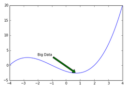
X = np.linspace(-4, 4, 1024)Y = .25 * (X + 4.) * (X + 1.) * (X - 2.)plt.annotate('Big Data',
ha ='center', va ='bottom',xytext =(-1.5, 3.0), xy =(0.75, -2.7),
arrowprops ={'facecolor': 'green', 'shrink':0.05, 'edgecolor': 'black'}) #arrow propertiesplt.plot(X, Y)

Out[76]:

[<matplotlib.lines.Line2D at 0x9d1def0>]

In [74]:

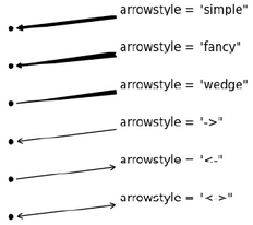
#arrow styles are :from IPython.display import ImageImage(filename='arrows.png')

Out[74]:

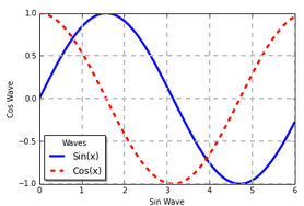
Legend properties:
'loc': This is the location of the legend. The default value is 'best', which will place it automatically. Other valid values are
'upper left', 'lower left', 'lower right', 'right', 'center left', 'center right', 'lower center', 'upper center', and 'center'.

'shadow': This can be either True or False, and it renders the legend with a shadow effect.

'fancybox': This can be either True or False and renders the legend with a rounded box.

'title': This renders the legend with the title passed as a parameter.

'ncol': This forces the passed value to be the number of columns for the legend

In [101]:

x =np.linspace(0, 6,1024)y1 =np.sin(x)y2 =np.cos(x)plt.xlabel('Sin Wave')plt.ylabel('Cos Wave')plt.plot(x, y1, c='b', lw =3.0, label ='Sin(x)') # labels are specifiedplt.plot(x, y2, c ='r', lw =3.0, ls ='--', label ='Cos(x)')plt.legend(loc ='best', shadow = True, fancybox = False, title ='Waves', ncol =1) # displays the labelsplt.grid(True, lw = 2, ls ='--', c='.75') # adds grid lines to the figureplt.show()

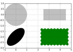
Shapes

In [4]:

#Paths for several kinds of shapes are available in the matplotlib.patches moduleimport matplotlib.patches as patchesdis = patches.Circle((0,0), radius = 1.0, color ='.75' )plt.gca().add_patch(dis) # used to render the image.dis = patches.Rectangle((2.5, -.5), 2.0, 1.0, color ='.75') #patches.rectangle((x & y coordinates), length, breadth)plt.gca().add_patch(dis)dis = patches.Ellipse((0, -2.0), 2.0, 1.0, angle =45, color ='.00')plt.gca().add_patch(dis)dis = patches.FancyBboxPatch((2.5, -2.5), 2.0, 1.0, boxstyle ='roundtooth', color ='g')plt.gca().add_patch(dis)plt.grid(True)plt.axis('scaled') # displays the images within the prescribed axisplt.show()#FancyBox: This is like a rectangle but takes an additional boxstyle parameter
#(either 'larrow', 'rarrow', 'round', 'round4', 'roundtooth', 'sawtooth', or 'square')

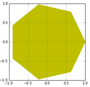
In [22]:

import matplotlib.patches as patchestheta = np.linspace(0, 2 * np.pi, 8) # generates an arrayvertical = np.vstack((np.cos(theta), np.sin(theta))).transpose() # vertical stack clubs the two arrays.
#print vertical, print and see how the array looksplt.gca().add_patch(patches.Polygon(vertical, color ='y'))plt.axis('scaled')plt.grid(True)plt.show()#The matplotlib.patches.Polygon()constructor takes a list of coordinates as the inputs, that is, the vertices of the polygon


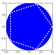
In [34]:

# a polygon can be imbided into a circletheta = np.linspace(0, 2 * np.pi, 6) # generates an arrayvertical = np.vstack((np.cos(theta), np.sin(theta))).transpose() # vertical stack clubs the two arrays.
#print vertical, print and see how the array looksplt.gca().add_patch(plt.Circle((0,0), radius =1.0, color ='b'))plt.gca().add_patch(plt.Polygon(vertical, fill =None, lw =4.0, ls ='dashed', edgecolor ='w'))plt.axis('scaled')plt.grid(True)plt.show()

Ticks in Matplotlib

In [54]:

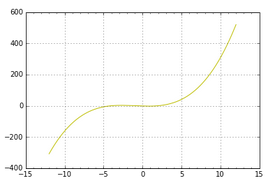
#In matplotlib, ticks are small marks on both the axes of a figureimport matplotlib.ticker as tickerX = np.linspace(-12, 12, 1024)Y = .25 * (X + 4.) * (X + 1.) * (X - 2.)pl =plt.axes() #the object that manages the axes of a figurepl.xaxis.set_major_locator(ticker.MultipleLocator(5))pl.xaxis.set_minor_locator(ticker.MultipleLocator(1))plt.plot(X, Y, c = 'y')plt.grid(True, which ='major') # which can take three values: minor, major and bothplt.show()

In [59]:

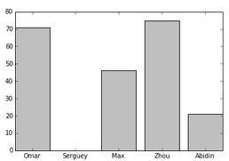
name_list = ('Omar', 'Serguey', 'Max', 'Zhou', 'Abidin')value_list = np.random.randint(0, 99, size = len(name_list))pos_list = np.arange(len(name_list))ax = plt.axes()ax.xaxis.set_major_locator(ticker.FixedLocator((pos_list)))ax.xaxis.set_major_formatter(ticker.FixedFormatter((name_list)))plt.bar(pos_list, value_list, color = '.75',align = 'center')plt.show()

MatplotLib Part3
4th 部分:

包含了一些復(fù)雜圖形。
Working with figures

In [4]:

%matplotlib inlineimport numpy as npimport matplotlib.pyplot as plt

In [5]:

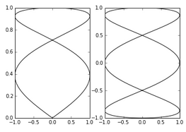
T = np.linspace(-np.pi, np.pi, 1024) #fig, (ax0, ax1) = plt.subplots(ncols =2)ax0.plot(np.sin(2 * T), np.cos(0.5 * T), c = 'k')ax1.plot(np.cos(3 * T), np.sin(T), c = 'k')plt.show()

Setting aspect ratio

In [7]:

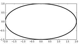
T = np.linspace(0, 2 * np.pi, 1024)plt.plot(2. * np.cos(T), np.sin(T), c = 'k', lw = 3.)plt.axes().set_aspect('equal') # remove this line of code and see how the figure looksplt.show()
 
In [12]:

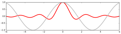
X = np.linspace(-6, 6, 1024)Y1, Y2 = np.sinc(X), np.cos(X)plt.figure(figsize=(10.24, 2.56)) #sets size of the figureplt.plot(X, Y1, c='r', lw = 3.)plt.plot(X, Y2, c='.75', lw = 3.)plt.show()

In [8]:

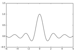
X = np.linspace(-6, 6, 1024)plt.ylim(-.5, 1.5)plt.plot(X, np.sinc(X), c = 'k')plt.show()

In [16]:

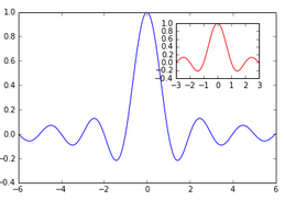
X = np.linspace(-6, 6, 1024)Y = np.sinc(X)X_sub = np.linspace(-3, 3, 1024)#coordinates of subplotY_sub = np.sinc(X_sub) # coordinates of sub plotplt.plot(X, Y, c = 'b')
sub_axes = plt.axes([.6, .6, .25, .25])# coordinates, length and width of the subplot framesub_axes.plot(X_detail, Y_detail, c = 'r')plt.show()

Log Scale

In [20]:

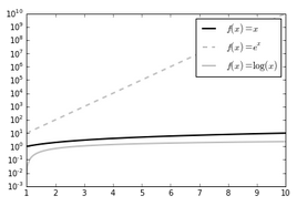
X = np.linspace(1, 10, 1024)plt.yscale('log') # set y scale as log. we would use plot.xscale()plt.plot(X, X, c = 'k', lw = 2., label = r'$f(x)=x$')plt.plot(X, 10 ** X, c = '.75', ls = '--', lw = 2., label = r'$f(x)=e^x$')plt.plot(X, np.log(X), c = '.75', lw = 2., label = r'$f(x)=\log(x)$')plt.legend()plt.show()#The logarithm base is 10 by default, but it can be changed with the optional parameters basex and basey.

Polar Coordinates

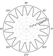
In [23]:

T = np.linspace(0 , 2 * np.pi, 1024)plt.axes(polar = True) # show polar coordinatesplt.plot(T, 1. + .25 * np.sin(16 * T), c= 'k')plt.show()

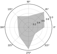
In [25]:
import matplotlib.patches as patches # import patch module from matplotlibax = plt.axes(polar = True)theta = np.linspace(0, 2 * np.pi, 8, endpoint = False)radius = .25 + .75 * np.random.random(size = len(theta))points = np.vstack((theta, radius)).transpose()plt.gca().add_patch(patches.Polygon(points, color = '.75'))plt.show()

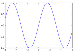
In [2]:
x = np.linspace(-6,6,1024)y= np.sin(x)plt.plot(x,y)plt.savefig('bigdata.png', c= 'y', transparent = True) #savefig function writes that data to a file# will create a file named bigdata.png. Its resolution will be 800 x 600 pixels, in 8-bit colors (24-bits per pixel)

In [3]:
theta =np.linspace(0, 2 *np.pi, 8)points =np.vstack((np.cos(theta), np.sin(theta))).Tplt.figure(figsize =(6.0, 6.0))plt.gca().add_patch(plt.Polygon(points, color ='r'))plt.axis('scaled')plt.grid(True)plt.savefig('pl.png', dpi =300) # try 'pl.pdf', pl.svg'#dpi is dots per inch. 300*8 x 6*300 = 2400 x 1800 pixels
MatplotLib Part4
總結(jié)
你學(xué)習(xí)Python時(shí)能犯的最簡單的錯(cuò)誤之一就是同時(shí)去嘗試學(xué)習(xí)過多的庫。當(dāng)你努力一下子學(xué)會每樣?xùn)|西時(shí)，你會花費(fèi)很多時(shí)間來切換這些不同概念之間，變得沮喪，最后轉(zhuǎn)移到其他事情上。