機器學習之Logistic回歸與Python實現

logistic回歸是一種廣義的線性回歸，通過構造回歸函數，利用機器學習來實現分類或者預測。

一 Logistic回歸概述

Logistic回歸的主要思想是，根據現有的數據對分類邊界建立回歸公式，從而實現分類（一般兩類）。“回歸”的意思就是要找到最佳擬合參數，其中涉及的數學原理和步驟如下：
（1）需要一個合適的分類函數來實現分類【單位階躍函數、Sigmoid函數】
（2）損失函數（Cost函數）來表示預測值（h(x)）與實際值(y)的偏差(h?y),要使得回歸最佳擬合，那么偏差要盡可能?。?a href='/map/piancha/' style='color:#000;font-size:inherit;'>偏差求和或取均值）。
（3）記J(ω)表示回歸系數為ω時的偏差，那么求最佳回歸參數ω就轉換成了求J(ω)的最小值?！?a href='/map/tiduxiajiang/' style='color:#000;font-size:inherit;'>梯度下降法】
所以，接下來就圍繞這幾個步驟進行展開。

1.1 分類函數

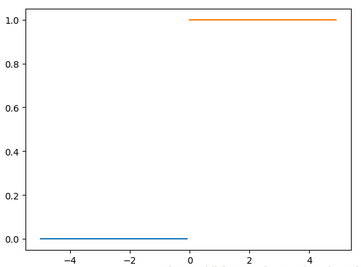
假設要實現二分類，那么可以找一個函數，根據不同的特征變量，輸出0和1，并且只輸出0和1，這種函數在某個點直接從0跳躍到1，如：
 
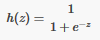
但是這種函數處理起來，稍微有點麻煩，我們選擇另外一個連續(xù)可導的函數，也就是Sigmoid函數,函數的公式如下：

這個函數的特點是，當x=0.5時，h(x)=0.5，而x越大，h(x)越接近1，x越小，h(x)越接近0。函數圖如下：

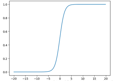
這個函數很像階躍函數，當x>0.5，就可以將數據分入1類；當x<0.5，就可以將數據分入0類。

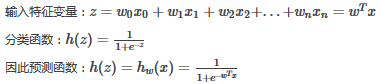
確定了分類函數，接下來，我們將Sigmoid函數的輸入記為z，那么

向量x是特征變量，是輸入數據，向量w是回歸系數是特征
之后的事情就是如何確定最佳回歸系數ω(w0,w1,w2,...,wn)

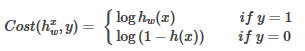
1.2 Cost函數

現有

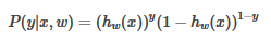
對于任意確定的x和w,有：

這個函數可以寫成：

取似然函數：

求對數似然函數：

因此，就構造得到了函數J(w)來表示預測值與實際值的偏差，于是Cost函數也可以寫成：

所以，我們可以用J(w)來表示預測值與實際值的偏差，也就是Cost函數，接下里的任務，就是如何讓偏差最小，也就是J(w)最大

Question:為什么J(w)可以表示預測值與實際值的大小，為什么J(w)最大表示偏差最小。

我們回到J(w)的推導來源，來自
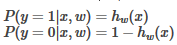
P(y=1|x,w)=hw(x)和P(y=0|x,w)=1?hw(x)，
那么顯然有
當x>0,此時y=1，1/2<hw(x)<1，所以P(y=1|x,w)=hw(x)>1/2
當x<0,此時y=0，0<hw(x)<1/2，所以P(y=0|x,w)=1?hw(x)>1/2
所以，無論如何取值，P(y=0|x,w)都大于等于1/2,P(y=0|x,w)越大，越接近1，表示落入某分類概率越大，那么分類越準確，預測值與實際值差異就越小。
所以P(y=0|x,w)可以表示預測值與實際值的差異，且P(y=0|x,w)越大表示差異越小，所以其似然函數J(w)越大，預測越準確。

所以，接下來的任務，是如何求解J(w)最大時的w值，其方法是梯度上升法。

1.3 梯度上升法求J(w)最大值

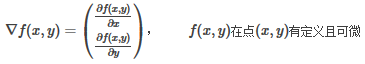
梯度上升法的核心思想是：要找某個函數的最大值，就沿著這個函數梯度方向探尋，如果梯度記為?，那么函數f(x,y)的梯度是：

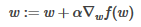
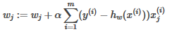
梯度上升法中，梯度算子沿著函數增長最快的方向移動（移動方向），如果移動大小為α（步長），那么梯度上升法的迭代公式是：

問題轉化成：

首先，我們對J(w)求偏導：

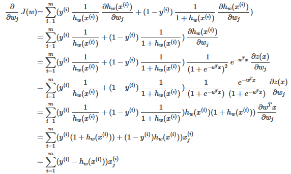
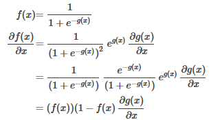
在第四至第五行的轉換，用到的公式是：

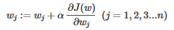
將求得的偏導公式代入梯度上升法迭代公示：

可以看到，式子中所有函數和輸入的值，都是已知的了。接下來，可以通過Python實現Logistic回歸了。

二、Python算法實現

2.1 梯度上升法求最佳回歸系數

首先，數據取自《機器學習實戰(zhàn)》中的數據，部分數據如下：

-0.017612   14.053064   0
-1.395634   4.662541    1
-0.752157   6.538620    0
-1.322371   7.152853    0
0.423363    11.054677   0
0.406704    7.067335    1

先定義函數來獲取數去，然后定義分類函數Sigmoid函數，最后利用梯度上升法求解回歸系數w。
建立一個logRegres.py文件，輸入如下代碼：

from numpy import *
#構造函數來獲取數據
def loadDataSet():
    dataMat=[];labelMat=[]
    fr=open('machinelearninginaction/Ch05/testSet.txt')
    for line in fr.readlines():
        lineArr=line.strip().split()
        dataMat.append([1.0,float(lineArr[0]),float(lineArr[1])])#特征數據集，添加1是構造常數項x0
        labelMat.append(int(lineArr[-1]))#分類數據集
    return dataMat,labelMat

def sigmoid(inX):
    return 1/(1+exp(-inX))

def gradAscent(dataMatIn,classLabels):
    dataMatrix=mat(dataMatIn) #(m,n)
    labelMat=mat(classLabels).transpose() #轉置后(m,1)
    m,n=shape(dataMatrix)
    weights=ones((n,1)) #初始化回歸系數，(n,1)
    alpha=0.001 #定義步長
    maxCycles=500 #定義最大循環(huán)次數
    for i in range(maxCycles):
        h=sigmoid(dataMatrix * weights) #sigmoid 函數
        error=labelMat - h #即y-h，（m,1）
        weights=weights + alpha * dataMatrix.transpose() * error #梯度上升法
    return weights

在python命令符中輸入代碼對函數進行測試：
In [8]: import logRegres
   ...:
In [9]: dataArr,labelMat=logRegres.loadDataSet()
   ...:
In [10]: logRegres.gradAscent(dataArr,labelMat)
    ...:
Out[10]:
matrix([[ 4.12414349],
        [ 0.48007329],
        [-0.6168482 ]])

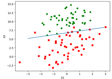
于是得到了回歸系數。接下來根據回歸系數畫出決策邊界wTx=0
定義作圖函數：

def plotBestFit(weights):
    import matplotlib.pyplot as plt
    dataMat,labelMat=loadDataSet()
    n=shape(dataMat)[0]
    xcord1=[];ycord1=[]
    xcord2=[];ycord2=[]
    for i in range(n):
        if labelMat[i]==1:
            xcord1.append(dataMat[i][1])
            ycord1.append(dataMat[i][2])
        else:
            xcord2.append(dataMat[i][1])
            ycord2.append(dataMat[i][2])
    fig=plt.figure()
    ax=fig.add_subplot(111)
    ax.scatter(xcord1,ycord1,s=30,c='red',marker='s')
    ax.scatter(xcord2,ycord2,s=30,c='green')
    x=arange(-3,3,0.1)
    y=(-weights[0,0]-weights[1,0]*x)/weights[2,0] #matix
    ax.plot(x,y)
    plt.xlabel('X1')
    plt.ylabel('X2')
    plt.show()

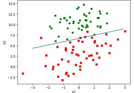
在Python的shell中對函數進行測試：

In [11]: weights=logRegres.gradAscent(dataArr,labelMat)

In [12]: logRegres.plotBestFit(weights)
    ...:

2.2 算法改進

(1) 隨機梯度上升
上述算法，要進行maxCycles次循環(huán)，每次循環(huán)中矩陣會有m*n次乘法計算，所以時間復雜度（開銷）是maxCycles*m*n，當數據量較大時，時間復雜度就會很大。因此，可以是用隨機梯度上升法來進行算法改進。

隨機梯度上升法的思想是，每次只使用一個數據樣本點來更新回歸系數。這樣就大大減小計算開銷。
代碼如下：

def stocGradAscent(dataMatrix,classLabels):
    m,n=shape(dataMatrix)
    alpha=0.01
    weights=ones(n)
    for i in range(m):
        h=sigmoid(sum(dataMatrix[i] * weights))#數值計算
        error = classLabels[i]-h
        weights=weights + alpha * error * dataMatrix[i] #array 和list矩陣乘法不一樣
    return weights

注意：gradAscent函數和這個stocGradAscent函數中的h和weights的計算形式不一樣，因為
前者是的矩陣的計算，類型是numpy的matrix，按照矩陣的運算規(guī)則進行計算。
后者是數值計算，其類型是list，按照數值運算規(guī)則計算。

對隨機梯度上升算法進行測試：

In [37]: dataMat,labelMat=logRegres.loadDataSet()
    ...:
In [38]: weights=logRegres.stocGradAscent(array(dataMat),labelMat)
    ...:
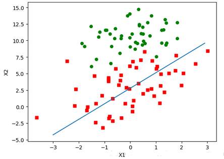
In [39]: logRegres.plotBestFit(mat(weights).transpose())
    ...:

輸出的樣本數據點和決策邊界是：

（2）改進的隨機梯度上升法

def stocGradAscent1(dataMatrix,classLabels,numIter=150):
    m,n=shape(dataMatrix)
    weights=ones(n)
    for j in range(numIter):
        dataIndex=list(range(m))
        for i in range(m):
            alpha=4/(1+i+j)+0.01#保證多次迭代后新數據仍然具有一定影響力
            randIndex=int(random.uniform(0,len(dataIndex)))#減少周期波動
            h=sigmoid(sum(dataMatrix[randIndex] * weights))
            error=classLabels[randIndex]-h
            weights=weights + alpha*dataMatrix[randIndex]*error
            del(dataIndex[randIndex])
    return weights 

在Python命令符中測試函數并畫出分類邊界：

In [188]: weights=logRegres.stocGradAscent1(array(dataMat),labelMat)
     ...:
In [189]: logRegres.plotBestFit(mat(weights).transpose())
     ...:

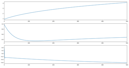
（3）三種方式回歸系數波動情況
普通的梯度上升法：
 
隨機梯度上升：
 
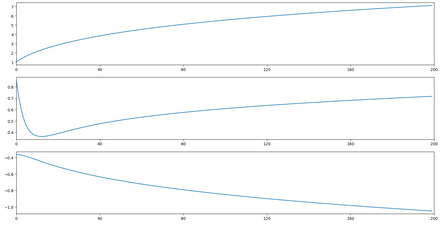
改進的隨機梯度上升

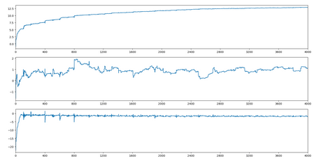
評價算法優(yōu)劣勢看它是或否收斂，是否達到穩(wěn)定值，收斂越快，算法越優(yōu)。

三 實例

3.1 通過logistic回歸和氙氣病癥預測馬的死亡率

數據取自《機器學習實戰(zhàn)》一書中的氙氣病癥與馬死亡的數據，部分數據如下：

2.000000    1.000000    38.500000   66.000000   28.000000   3.000000    3.000000    0.000000    2.000000    5.000000    4.000000    4.000000    0.000000    0.000000    0.000000    3.000000    5.000000    45.000000   8.400000    0.000000    0.000000    0.000000
1.000000    1.000000    39.200000   88.000000   20.000000   0.000000    0.000000    4.000000    1.000000    3.000000    4.000000    2.000000    0.000000    0.000000    0.000000    4.000000    2.000000    50.000000   85.000000   2.000000    2.000000    0.000000
2.000000    1.000000    38.300000   40.000000   24.000000   1.000000    1.000000    3.000000    1.000000    3.000000    3.000000    1.000000    0.000000    0.000000    0.000000    1.000000    1.000000    33.000000   6.700000    0.000000    0.000000    1.000000

通過21個特征數據，來對結果進行分類和預測。

#定義分類函數，prob>0.5，則分入1，否則分類0
def classifyVector(inX,trainWeights):
    prob=sigmoid(sum(inX*trainWeights))
    if prob>0.5:return 1
    else : return 0

def colicTest():
    frTrain = open('machinelearninginaction/Ch05/horseColicTraining.txt')#訓練數據
    frTest = open('machinelearninginaction/Ch05/horseColicTest.txt')#測試數據
    trainSet=[];trainLabels=[]
    for line in frTrain.readlines():
        currLine=line.strip().split('\t')
        lineArr=[]
        for i in range(21):
            lineArr.append(float(currLine[i]))
        trainSet.append(lineArr)
        trainLabels.append(float(currLine[21]))
    trainWeights=stocGradAscent1(array(trainSet),trainLabels,500)#改進的隨機梯度上升法
    errorCount=0;numTestVec=0
    for line in frTest.readlines():
        numTestVec+=1
        currLine=line.strip().split('\t')
        lineArr=[]
        for i in range(21):
            lineArr.append(float(currLine[i]))
        if classifyVector(array(lineArr),trainWeights)!=int(currLine[21]):
            errorCount+=1
    errorRate=(float(errorCount)/numTestVec)
    print('the error rate of this test is :%f'%errorRate)
    return errorRate
def multiTest():#進行多次測試
    numTests=10;errorSum=0
    for k in range(numTests):
        errorSum+=colicTest()
    print('after %d iterations the average error rate is:%f'%(numTests,errorSum/float(numTests)))

在控制臺命令符中輸入命令來對函數進行測試：

In [3]: logRegres.multiTest()
G:\Workspaces\MachineLearning\logRegres.py:19: RuntimeWarning: overflow encountered in exp
  return 1/(1+exp(-inX))
the error rate of this test is :0.313433
the error rate of this test is :0.268657
the error rate of this test is :0.358209
the error rate of this test is :0.447761
the error rate of this test is :0.298507
the error rate of this test is :0.373134
the error rate of this test is :0.358209
the error rate of this test is :0.417910
the error rate of this test is :0.432836
the error rate of this test is :0.417910
after 10 iterations the average error rate is:0.368657

分類的錯誤率是36.9%。