用R語言做邏輯回歸

回歸的本質是建立一個模型用來預測，而邏輯回歸的獨特性在于，預測的結果是只能有兩種，true or false
在R里面做邏輯回歸也很簡單，只需要構造好數(shù)據(jù)集，然后用glm函數(shù)(廣義線性模型（generalized linear model）)建模即可,預測用predict函數(shù)。
我這里簡單講一個例子，來自于加州大學洛杉磯分校的課程
首先加載需要用的包
library(ggplot2)
library(Rcpp)
然后加載測試數(shù)據(jù)
mydata <- read.csv("http://www.ats.ucla.edu/stat/data/binary.csv") ## 這里直接讀取網(wǎng)絡數(shù)據(jù)head(mydata)
##   admit gre  gpa rank
## 1     0 380 3.61    3
## 2     1 660 3.67    3
## 3     1 800 4.00    1
## 4     1 640 3.19    4
## 5     0 520 2.93    4
## 6     1 760 3.00    2
#This dataset has a binary response (outcome, dependent) variable called admit.

#There are three predictor variables: gre, gpa and rank. We will treat the variables gre and gpa as continuous.

#The variable rank takes on the values 1 through 4.

summary(mydata)
##      admit             gre             gpa             rank      
##  Min.   :0.0000   Min.   :220.0   Min.   :2.260   Min.   :1.000  
##  1st Qu.:0.0000   1st Qu.:520.0   1st Qu.:3.130   1st Qu.:2.000  
##  Median :0.0000   Median :580.0   Median :3.395   Median :2.000  
##  Mean   :0.3175   Mean   :587.7   Mean   :3.390   Mean   :2.485  
##  3rd Qu.:1.0000   3rd Qu.:660.0   3rd Qu.:3.670   3rd Qu.:3.000  
##  Max.   :1.0000   Max.   :800.0   Max.   :4.000   Max.   :4.000
sapply(mydata, sd)
##       admit         gre         gpa        rank
##   0.4660867 115.5165364   0.3805668   0.9444602
xtabs(~ admit + rank, data = mydata)  ##保證結果變量只能是錄取與否，不能有其它！?。?br /> ##      rank
## admit  1  2  3  4
##     0 28 97 93 55
##     1 33 54 28 12
可以看到這個數(shù)據(jù)集是關于申請學校是否被錄取的，根據(jù)學生的GRE成績，GPA和排名來預測該學生是否被錄取。

其中GRE成績是連續(xù)性的變量，學生可以考取任意正常分數(shù)。

而GPA也是連續(xù)性的變量，任意正常GPA均可。

最后的排名雖然也是連續(xù)性變量，但是一般前幾名才有資格申請，所以這里把它當做因子，只考慮前四名！

而我們想做這個邏輯回歸分析的目的也很簡單，就是想根據(jù)學生的成績排名，績點信息，托福或者GRE成績來預測它被錄取的概率是多少！

接下來建模
mydata$rank <- factor(mydata$rank)

mylogit <- glm(admit ~ gre + gpa + rank, data = mydata, family = "binomial")

summary(mylogit)
##
## Call:
## glm(formula = admit ~ gre + gpa + rank, family = "binomial",
##     data = mydata)
##
## Deviance Residuals:
##     Min       1Q   Median       3Q      Max  
## -1.6268  -0.8662  -0.6388   1.1490   2.0790  
##
## Coefficients:
##              Estimate Std. Error z value Pr(>|z|)    
## (Intercept) -3.989979   1.139951  -3.500 0.000465 ***
## gre          0.002264   0.001094   2.070 0.038465 *  
## gpa          0.804038   0.331819   2.423 0.015388 *  
## rank2       -0.675443   0.316490  -2.134 0.032829 *  
## rank3       -1.340204   0.345306  -3.881 0.000104 ***
## rank4       -1.551464   0.417832  -3.713 0.000205 ***
## ---
## Signif. codes:  0 '***' 0.001 '**' 0.01 '*' 0.05 '.' 0.1 ' ' 1
##
## (Dispersion parameter for binomial family taken to be 1)
##
##     Null deviance: 499.98  on 399  degrees of freedom
## Residual deviance: 458.52  on 394  degrees of freedom
## AIC: 470.52
##
## Number of Fisher Scoring iterations: 4
根據(jù)對這個模型的summary結果可知：

GRE成績每增加1分，被錄取的優(yōu)勢對數(shù)(log odds)增加0.002

而GPA每增加1單位，被錄取的優(yōu)勢對數(shù)(log odds)增加0.804，不過一般GPA相差都是零點幾。

最后第二名的同學比第一名同學在其它同等條件下被錄取的優(yōu)勢對數(shù)(log odds)小了0.675，看來排名非常重要啊?。?！

這里必須解釋一下這個優(yōu)勢對數(shù)(log odds)是什么意思了，如果預測這個學生被錄取的概率是p，那么優(yōu)勢對數(shù)(log odds)就是log2(p/(1-p)),一般是以自然對數(shù)為底

最后我們可以根據(jù)模型來預測啦
## 重點是predict函數(shù)，type參數(shù)

newdata1 <- with(mydata,                 
data.frame(gre = mean(gre), gpa = mean(gpa), rank = factor(1:4)))

newdata1
##     gre    gpa rank
## 1 587.7 3.3899    1
## 2 587.7 3.3899    2
## 3 587.7 3.3899    3
## 4 587.7 3.3899    4
## 這里構造一個需要預測的矩陣，4個學生，除了排名不一樣，GRE和GPA都一樣newdata1$rankP <- predict(mylogit, newdata = newdata1, type = "response")

newdata1
##     gre    gpa rank     rankP
## 1 587.7 3.3899    1 0.5166016
## 2 587.7 3.3899    2 0.3522846
## 3 587.7 3.3899    3 0.2186120
## 4 587.7 3.3899    4 0.1846684
## type = "response" 直接返回預測的概率值0~1之間
可以看到，排名越高，被錄取的概率越大?。?！

log(0.5166016/(1-0.5166016)) ## 第一名的優(yōu)勢對數(shù)0.06643082

log((0.3522846/(1-0.3522846))) ##第二名的優(yōu)勢對數(shù)-0.609012

兩者的差值正好是0.675，就是模型里面預測的！

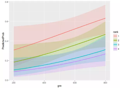
newdata2 <- with(mydata,                 data.frame(gre = rep(seq(from = 200, to = 800, length.out = 100), 4),                            gpa = mean(gpa), rank = factor(rep(1:4, each = 100))))##newdata2##這個數(shù)據(jù)集也是構造出來，需要用模型來預測的！newdata3 <- cbind(newdata2, predict(mylogit, newdata = newdata2, type="link", se=TRUE))## type="link" 返回fit值，需要進一步用plogis處理成概率值## ?plogis The Logistic Distributionnewdata3 <- within(newdata3, {
  PredictedProb <- plogis(fit)
  LL <- plogis(fit - (1.96 * se.fit))
  UL <- plogis(fit + (1.96 * se.fit))})
最后可以做一些簡單的可視化
head(newdata3)
##        gre    gpa rank        fit    se.fit residual.scale        UL
## 1 200.0000 3.3899    1 -0.8114870 0.5147714              1 0.5492064
## 2 206.0606 3.3899    1 -0.7977632 0.5090986              1 0.5498513
## 3 212.1212 3.3899    1 -0.7840394 0.5034491              1 0.5505074
## 4 218.1818 3.3899    1 -0.7703156 0.4978239              1 0.5511750
## 5 224.2424 3.3899    1 -0.7565919 0.4922237              1 0.5518545
## 6 230.3030 3.3899    1 -0.7428681 0.4866494              1 0.5525464
##          LL PredictedProb
## 1 0.1393812     0.3075737
## 2 0.1423880     0.3105042
## 3 0.1454429     0.3134499
## 4 0.1485460     0.3164108
## 5 0.1516973     0.3193867
## 6 0.1548966     0.3223773
ggplot(newdata3, aes(x = gre, y = PredictedProb)) +
  geom_ribbon(aes(ymin = LL, ymax = UL, fill = rank), alpha = .2) +
  geom_line(aes(colour = rank), size=1)