用十張圖解釋機(jī)器學(xué)習(xí)的基本概念

在解釋機(jī)器學(xué)習(xí)的基本概念的時候，我發(fā)現(xiàn)自己總是回到有限的幾幅圖中。以下是我認(rèn)為最有啟發(fā)性的條目列表。

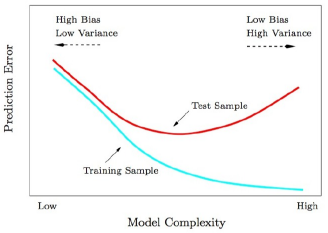
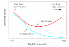
1. Test and training error: 為什么低訓(xùn)練誤差并不總是一件好的事情呢：ESL 圖2.11.以模型復(fù)雜度為變量的測試及訓(xùn)練錯誤函數(shù)。

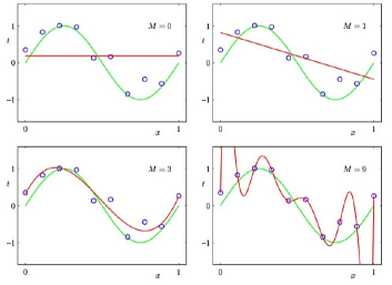
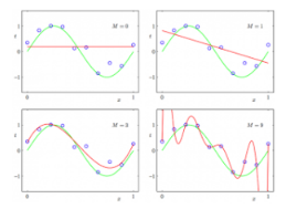
2. Under and overfitting: 低度擬合或者過度擬合的例子。PRML 圖1.4.多項式曲線有各種各樣的命令M，以紅色曲線表示，由綠色曲線適應(yīng)數(shù)據(jù)集后生成。

3. Occam’s razor

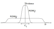
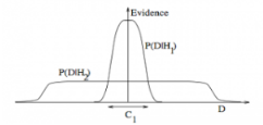
ITILA 圖28.3.為什么貝葉斯推理可以具體化奧卡姆剃刀原理。這張圖給了為什么復(fù)雜模型原來是小概率事件這個問題一個基本的直觀的解釋。水平軸代表了可能的數(shù)據(jù)集D空間。貝葉斯定理以他們預(yù)測的數(shù)據(jù)出現(xiàn)的程度成比例地反饋模型。這些預(yù)測被數(shù)據(jù)D上歸一化概率分布量化。數(shù)據(jù)的概率給出了一種模型Hi,P(D|Hi)被稱作支持Hi模型的證據(jù)。一個簡單的模型H1僅可以做到一種有限預(yù)測，以P(D|H1)展示；一個更加強(qiáng)大的模型H2，舉例來說，可以比模型H1擁有更加自由的參數(shù)，可以預(yù)測更多種類的數(shù)據(jù)集。這也表明，無論如何，H2在C1域中對數(shù)據(jù)集的預(yù)測做不到像H1那樣強(qiáng)大。假設(shè)相等的先驗概率被分配給這兩種模型，之后數(shù)據(jù)集落在C1區(qū)域，不那么強(qiáng)大的模型H1將會是更加合適的模型。

4. Feature combinations：

(1)為什么集體相關(guān)的特征單獨來看時無關(guān)緊要，這也是（2）線性方法可能會失敗的原因。從Isabelle Guyon特征提取的幻燈片來看。

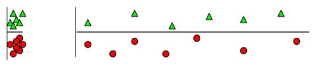
5. Irrelevant features:

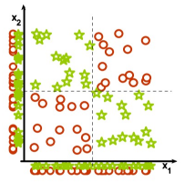
為什么無關(guān)緊要的特征會損害KNN，聚類，以及其它以相似點聚集的方法。左右的圖展示了兩類數(shù)據(jù)很好地被分離在縱軸上。右圖添加了一條不切題的橫軸，它破壞了分組，并且使得許多點成為相反類的近鄰。

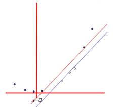
6. Basis functions

非線性的基礎(chǔ)函數(shù)是如何使一個低維度的非線性邊界的分類問題，轉(zhuǎn)變?yōu)橐粋€高維度的線性邊界問題。Andrew Moore的支持向量機(jī)SVM(Support Vector Machine)教程幻燈片中有：一個單維度的非線性帶有輸入x的分類問題轉(zhuǎn)化為一個2維的線性可分的z=(x,x^2)問題。

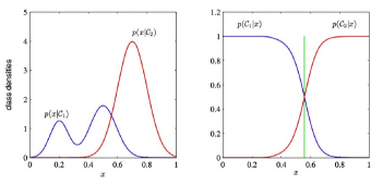
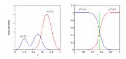
7. Discriminative vs. Generative:

為什么判別式學(xué)習(xí)比產(chǎn)生式更加簡單：PRML 圖1.27.這兩類方法的分類條件的密度舉例，有一個單一的輸入變量x（左圖），連同相應(yīng)的后驗概率（右圖）。注意到左側(cè)的分類條件密度p(x|C1)的模式，在左圖中以藍(lán)色線條表示，對后驗概率沒有影響。右圖中垂直的綠線展示了x中的決策邊界，它給出了最小的誤判率。

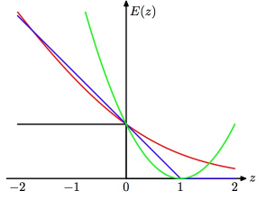
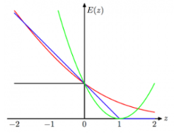
8. Loss functions:

學(xué)習(xí)算法可以被視作優(yōu)化不同的損失函數(shù)：PRML 圖7.5. 應(yīng)用于支持向量機(jī)中的“鉸鏈”錯誤函數(shù)圖形，以藍(lán)色線條表示，為了邏輯回歸，隨著錯誤函數(shù)被因子1/ln(2)重新調(diào)整，它通過點（0，1），以紅色線條表示。黑色線條表示誤分，均方誤差以綠色線條表示。

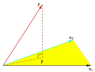
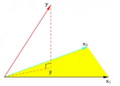
9. Geometry of least squares:

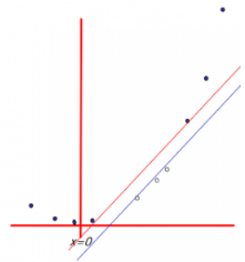
ESL 圖3.2.帶有兩個預(yù)測的最小二乘回歸的N維幾何圖形。結(jié)果向量y正交投影到被輸入向量x1和x2所跨越的超平面。投影y^代表了最小二乘預(yù)測的向量。

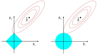
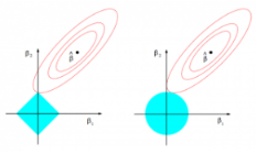
10. Sparsity:

為什么Lasso算法（L1正規(guī)化或者拉普拉斯先驗）給出了稀疏的解決方案（比如：帶更多0的加權(quán)向量）：ESL 圖3.11.lasso算法的估算圖像(左)以及嶺回歸算法的估算圖像（右）。展示了錯誤的等值線以及約束函數(shù)。分別的，當(dāng)紅色橢圓是最小二乘誤差函數(shù)的等高線時，實心的藍(lán)色區(qū)域是約束區(qū)域|β1| + |β2| ≤ t以及β12 + β22 ≤ t2。數(shù)據(jù)分析師培訓(xùn)

英文原文：

I find myself coming back to the same few pictures when explaining basic machine learning concepts. Below is a list I find most illuminating.

我發(fā)現(xiàn)自己在解釋基本的機(jī)器學(xué)習(xí)概念時經(jīng)常碰到少數(shù)相同的圖片。下面列舉了我認(rèn)為最有啟發(fā)性的圖片。

1. Test and training error(測試和訓(xùn)練錯誤): Why lower training error is not always a good thing: ESL Figure 2.11. Test and training error as a function of model complexity.

2. Under and overfitting(欠擬合和過擬合): PRML Figure 1.4. Plots of polynomials having various orders M, shown as red curves, fitted to the data set generated by the green curve.

3. Occam’s razor(奧卡姆剃刀): ITILA Figure 28.3. Why Bayesian inference embodies Occam’s razor. This figure gives the basic intuition for why complex models can turn out to be less probable. The horizontal axis represents the space of possible data sets D. Bayes’ theorem rewards models in proportion to how much they predicted the data that occurred. These predictions are quantified by a normalized probability distribution on D. This probability of the data given model Hi, P (D | Hi), is called the evidence for Hi. A simple model H1 makes only a limited range of predictions, shown by P(D|H1); a more powerful model H2, that has, for example, more free parameters than H1, is able to predict a greater variety of data sets. This means, however, that H2 does not predict the data sets in region C1 as strongly as H1. Suppose that equal prior probabilities have been assigned to the two models. Then, if the data set falls in region C1, the less powerful model H1 will be the more probable model.

4. Feature combinations(Feature組合): (1) Why collectively relevant features may look individually irrelevant, and also (2) Why linear methods may fail. From Isabelle Guyon’s feature extraction slides.

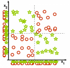
5. Irrelevant features(不相關(guān)特征): Why irrelevant features hurt kNN, clustering, and other similarity based methods. The figure on the left shows two classes well separated on the vertical axis. The figure on the right adds an irrelevant horizontal axis which destroys the grouping and makes many points nearest neighbors of the opposite class.

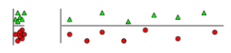
6. Basis functions(基函數(shù)): How non-linear basis functions turn a low dimensional classification problem without a linear boundary into a high dimensional problem with a linear boundary. From SVM tutorial slides by Andrew Moore: a one dimensional non-linear classification problem with input x is turned into a 2-D problem z=(x, x^2) that is linearly separable.

7. Discriminative vs. Generative(判別與生成): Why discriminative learning may be easier than generative: PRML Figure 1.27. Example of the class-conditional densities for two classes having a single input variable x (left plot) together with the corresponding posterior probabilities (right plot). Note that the left-hand mode of the class-conditional density p(x|C1), shown in blue on the left plot, has no effect on the posterior probabilities. The vertical green line in the right plot shows the decision boundary in x that gives the minimum misclassification rate.

8. Loss functions(損失函數(shù)): Learning algorithms can be viewed as optimizing different loss functions: PRML Figure 7.5. Plot of the ‘hinge’ error function used in support vector machines, shown in blue, along with the error function for logistic regression, rescaled by a factor of 1/ln(2) so that it passes through the point (0, 1), shown in red. Also shown are the misclassification error in black and the squared error in green.

9. Geometry of least squares(最小二乘的幾何圖形): ESL Figure 3.2. The N-dimensional geometry of least squares regression with two predictors. The outcome vector y is orthogonally projected onto the hyperplane spanned by the input vectors x1 and x2. The projection y? represents the vector of the least squares predictions.

10. Sparsity(稀疏性): Why Lasso (L1 regularization or Laplacian prior) gives sparse solutions (i.e. weight vectors with more zeros): ESL Figure 3.11. Estimation picture for the lasso (left) and ridge regression (right). Shown are contours of the error and constraint functions. The solid blue areas are the constraint regions |β1| + |β2| ≤ t and β12 + β22 ≤ t2, respectively, while the red ellipses are the contours of the least squares error function.